Improper Integrals and Other Discontinuities 1
6.9 Improper Integrals and Other
Discontinuities
In Exercises 1 – 3:
(a) Compute the value of the indicated definite integral using the trapezoidal
rule, Simpson’s rule, the Midpoint Rule and the two-point Gaussian quadrature
rule, programming the integrand as given. Use n= 2, 4, 8, 16, 32 and 64 for
each method. Compare the observed order of convergence with the theoretical
value.
(b) Repeat part (a) after making an appropriate change of variable in the inte-
grand.
1. R1
0e√xdx
(a) The table below lists the error in the approximate value of
Trapezoidal Simpson’s Midpoint Two-point
nRule Rule Rule Gaussian
2 5.637 ×10−22.821 ×10−21.308 ×10−22.536 ×10−3
8 8.902 ×10−33.575 ×10−32.147 ×10−33.210 ×10−4
2Section 6.9
(b) With the change of variable x=u2,
The table below lists the error in the approximate value of the transformed
integral computed using the trapezoidal rule, Simpson’s rule, the Midpoint
Trapezoidal Simpson’s Midpoint Two-point
nRule Rule Rule Gaussian
4 4.613 ×10−23.381 ×10−42.303 ×10−21.420 ×10−5
16 2.888 ×10−31.334 ×10−61.444 ×10−35.561 ×10−8
Order of Convergence:
2. R1
0x5/2dx
(a) The table below lists the error in the approximate value of
Improper Integrals and Other Discontinuities 3
Trapezoidal Simpson’s Midpoint Two-point
nRule Rule Rule Gaussian
2 5.267 ×10−21.196 ×10−32.652 ×10−27.648 ×10−5
8 3.260 ×10−31.180 ×10−51.632 ×10−37.023 ×10−7
(b) With the change of variable x=u2,
Trapezoidal Simpson’s Midpoint Two-point
nRule Rule Rule Gaussian
4 6.121 ×10−24.976 ×10−33.012 ×10−22.144 ×10−4
Order of Convergence:
3. R1
0sin(√x)dx
(a) The table below lists the error in the approximate value of
4Section 6.9
Trapezoidal Simpson’s Midpoint Two-point
nRule Rule Rule Gaussian
2 6.715 ×10−22.900 ×10−21.826 ×10−22.611 ×10−3
Order of Convergence:
(b) With the change of variable x=u2,
Trapezoidal Simpson’s Midpoint Two-point
nRule Rule Rule Gaussian
4 1.443 ×10−21.346 ×10−47.226 ×10−35.559 ×10−6
16 8.997 ×10−45.200 ×10−74.499 ×10−42.165 ×10−8
For the integrals given in Exercises 4 – 13, identify each discontinuity/limit of
integration which must be handled, then take appropriate action, and compute
the value of the integral, accurate to at least ten decimal places.
4. R1
0
sin x
xdx
Improper Integrals and Other Discontinuities 5
The integrand is discontinuous at the lower limit of integration, x= 0. Because
5. R1
0
x1/7
1+x2dx
Derivatives of the integrand are discontinuous at the lower limit of integration,
x= 0. Making the change of variable x=u7,
6. R1
0
ln(1−x)
√xdx
Here, the integrand has an algebraic discontinuity at the lower limit of integration,
x= 0, and a logarithmic discontinuity at the upper limit of integration, x= 1.
Let’s split the integration interval at x= 1/2. For
6Section 6.9
the discontinuous behavior of the integrand is controlled by ln(1 −x). Subtracting
away the discontinuous behavior, we rewrite this portion of the problem as
In the former integral, the logarithmic discontinuity has been replaced by a remov-
able discontinuity. Programming the integrand as the piecewise function
and using the adaptive three-point Gaussian quadrature rule with = 2.5×10⁻¹¹,
7. R∞
0e−x4dx
We handle the infinite upper limit of integration by breaking the integral into
Improper Integrals and Other Discontinuities 7
The discontinuity at u= 0 is removable with
8. R1
0
ex
√1−xdx
The integrand has an algebraic discontinuity at the upper limit of integration, x= 1.
9. R∞
0
dx
√x(x+1)
Here, we have an algebraic discontinuity at the lower limit of integration, x= 0,
where we have used the adaptive three-point Gaussian quadrature rule with =
8Section 6.9
Therefore,
10. R∞
0
dx
1+x3
We handle the infinite upper limit of integration by breaking the integral into
The first integral on the right-hand side is not improper and can be approximated
using the adaptive three-point Gaussian quadrature rule with = 2.5×10⁻¹¹. In
11. R1
0e−x2ln(1+x)
x2−1
xdx
The integrand is discontinuous at the lower limit of integration, x= 0. Because
Improper Integrals and Other Discontinuities 9
and using the adaptive Boole’s rule with = 5 ×10⁻¹¹, we find
12. R∞
1
e−x2ln(1+x)
x2dx
To eliminate the infinite upper limit of integration, we make the change of variable
13. R∞
−∞
x2
(x2+1)(x2−x+1) dx
To handle the infinite limits of integration, we make the change of variable x=
14. Compute the value of the integral
Z∞
1
ln x
1 + x2dx,
accurate to at least ten decimal places in two ways:
10 Section 6.9
(a) making the substitution x= 1/u; and
(b) making the substitution x= tan θ.
(a) Making the substitution x= 1/u, we find
In the text (just prior to Example 6.21), we found
(b) Making the substitution x= tan θ, we find
The latter integral can be evaluated analytically:
Improper Integrals and Other Discontinuities 11
and using the adaptive Boole’s rule with = 2.5×10⁻¹¹, we find
15. An integral of the form
Z1
−1
f(x)
√1−x2dx
has discontinuities at both endpoints of the integration interval. For integrals
of this type, the substitution x= sin θtransforms the problem to
Z1
−1
f(x)
√1−x2dx =Zπ/2
−π/2
f(sin θ)dθ.
Evaluate each of the following integrals using this approach.
(a) R1
−1
ex
√1−x2dx (b) R1
−1
x4
√1−x2dx (c) R1
−1
cos(πx)
√1−x2dx
(a) Let x= sin θ. Then
(b) Let x= sin θ. Then
(c) Let x= sin θ. Then
16. Repeat Exercise 15, but make the substitution x= cos θ.
(a) Let x= cos θ. Then
(b) Let x= cos θ. Then
(c) Let x= cos θ. Then
17. The integral
G(t) = Z∞
0
e−t/xe−x2/2dx
arises in studies of hopping transport for one-dimensional percolation (see J.
Bernasconi, “Hopping transport in one-dimensional percolation model: A com-
ment,” Phys. Rev. B, 25, 1982, pp. 1394-5). Evaluate G(1) and G(5).
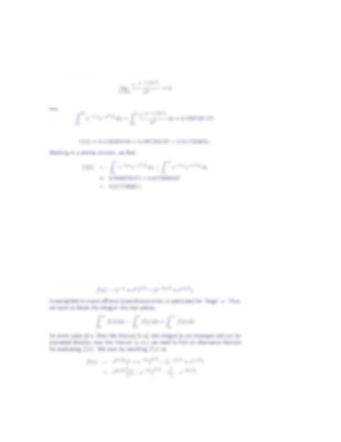
First write
Using the adaptive three-point Gaussian quadrature rule with = 2.5×10⁻¹¹, we
Improper Integrals and Other Discontinuities 13
The discontinuity at u= 0 is removable with
Using the adaptive three-point Gaussian quadrature rule with = 2.5×10⁻¹¹, we
Therefore,
18. In determining the overlap interaction for the kinetic energy of a free electron
gas, the integral
K(α) = Z∞
0(e−x+ex)α−(e−αx +eαx)dx
arises (see W. Harrison, “Total energies in the tight-binding theory,” Phys. Rev.
B, 23, 1981, pp. 5230 – 5245). In particular, the value of K(5/3) is needed.
Evaluate K(5/3).
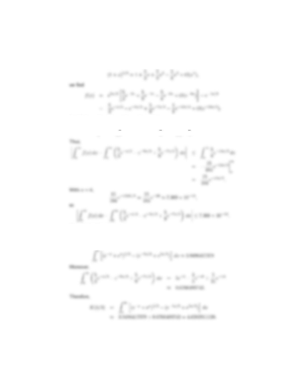
This problem is a bit tricky. In addition to the infinite upper limit of integration,
we need to be aware that evaluation of the integrand,
14 Section 6.9
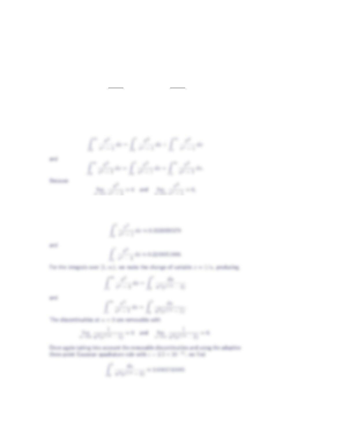
Using the series expansion for (1 + x)5/3:
As this is an alternating series, we know that
f(x)−5
3e−x/3−e−5x/3+5
9e−7x/3≤5
8e−13x/3.
We will therefore take a= 6.
Now, using the adaptive three-point Gaussian quadrature rule with = 2.5×10⁻¹¹,
we find
Improper Integrals and Other Discontinuities 15
19. Evaluate the integrals
Z∞
0
x2
ex−1dx and Z∞
0
x3
ex−1dx,
whise arise in determining the photon density and the energy density, respec-
tively, associated with blackbody radiation (see A. Beiser, Concepts of Modern
Physics, McGraw-Hill, New York, 1981).
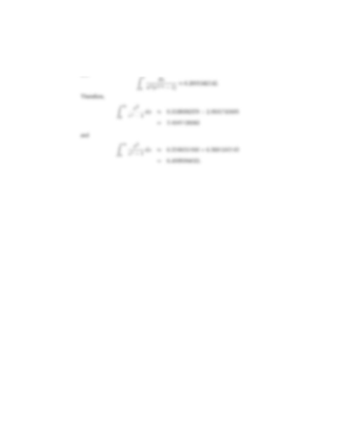
First, let’s rewrite the integrals as
the integrals over [0,1] have removable discontinuities at x= 0. Taking into
account the removable discontinuities and using the adaptive three-point Gaussian
quadrature rule with = 2.5×10⁻¹¹, we find
16 Section 6.9
and