Composite Newton-Cotes Quadrature 13
17. R2
1
sin x
xdx
Let f(x) = sin x
x. Then
For the the composite midpoint rule and the composite Simpson’s rule, the corre-
sponding inequalities are
respectively. The solutions of these inequalities are
18. R1
0
1
√1+x4dx
Let f(x) = 1
√1+x4. Then
For the the composite midpoint rule and the composite Simpson’s rule, the corre-
sponding inequalities are
14 Section 6.5
respectively. The solutions of these inequalities are
19. R4
0x√x2+ 9dx
Let f(x) = x√x2+ 9. Then
For the the composite midpoint rule and the composite Simpson’s rule, the corre-
sponding inequalities are
respectively. The solutions of these inequalities are
20. R1
0√1 + x3dx
Composite Newton-Cotes Quadrature 15
For the the composite midpoint rule and the composite Simpson’s rule, the corre-
sponding inequalities are
respectively. The solutions of these inequalities are
21. (a) Show that the error associated with the composite Simpson’s rule can be
approximated by
−h4
180 [f′′′(b)−f′′′(a)] .
(Hint: Recognize that 2hPm
j=1 f(4)(ξj) is a Riemann sum for Rb
af(4)(x)dx.)
(b) Show that the error associated with the composite midpoint rule can be
approximated by
h2
6[f′(b)−f′(a)] .
16 Section 6.5
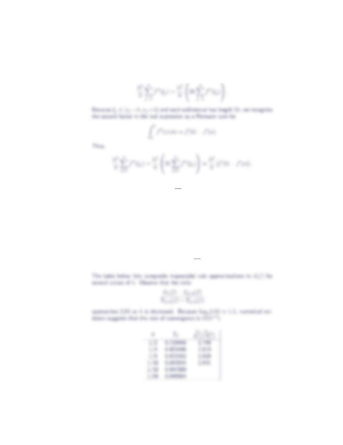
(b) First, rewrite the error term associated with the composite midpoint rule as
22. Consider the definite integral Rb
asin(√πx)dx. Numerically determine the rate
of convergence of the composite trapezoidal rule for each of the following inte-
gration intervals.
(a) [a, b] = [0,1] (b) [a, b] = [π/4,9π/4] (c) [a, b] = [π, 2π]
(d) Explain any variation among the rates of convergence obtained in parts
(a), (b) and (c).
(a) Consider the definite integral
I(f) = Z1
0
sin(√πx)dx.
Composite Newton-Cotes Quadrature 17
(b) Consider the definite integral
The table below lists composite trapezoidal rule approximations to I(f)for
several values of h. Observe that the ratio
(c) Consider the definite integral
The table below lists composite trapezoidal rule approximations to I(f)for
several values of h. Observe that the ratio
(d) The rate of convergence is lower than expected in part (a) because the deriva-
23. Repeat Exercise 22 for the composite midpoint rule.
(a) Consider the definite integral
The table below lists composite midpoint rule approximations to I(f)for sev-
eral values of h. Observe that the ratio
(b) Consider the definite integral
The table below lists composite midpoint rule approximations to I(f)for sev-
eral values of h. Observe that the ratio
approaches 16 as his decreased. Because 16 = 24, numerical evidence sug-
gests that the rate of convergence is O(h4).
hMh
Mh−Mh/2
Mh/2−Mh/4
1/2 −1.38405347794640 10.718
Composite Newton-Cotes Quadrature 19
(c) Consider the definite integral
I(f) = Z2π
π
sin(√πx)dx.
The table below lists composite midpoint rule approximations to I(f)for sev-
eral values of h. Observe that the ratio
hMh
Mh−Mh/2
Mh/2−Mh/4
1/2 −1.903034 4.066
(d) The rate of convergence is lower than expected in part (a) because the deriva-
24. Consider the definite integral R5/4
−1(x4+x3−3x2−4x−1)dx.
(a) Numerically determine the rate of convergence of the composite trapezoidal
rule when applied to the given integral.
(b) Numerically determine the rate of convergence of the composite midpoint
rule when applied to the given integral.
(c) Provide an explanation for the results obtained in parts (a) and (b).
Consider the definite integral
hTh|e2h/eh|
1/2 −5.27755737304690
hMh|e2h/eh|
1/2 −5.05230331420899
25. With an optimal tilting strategy, the theoretical lower bound for the time needed
to pour milk from a plastic pouch into a pitcher (N. Curle, “Liquid Flowing from
a Container,” in Mathematical Modeling, Andrews and McLone, eds., Butter-
worths, 1976, pp. 39 – 55) requires the calculation of the integrals
Z0.8355
0.1763
(1 + x2)1/4dx and Z1
0.8355
2 + x2
x3(1 + x2)1/4dx.
Approximate the value of each integral with an absolute error no greater than
10−4.
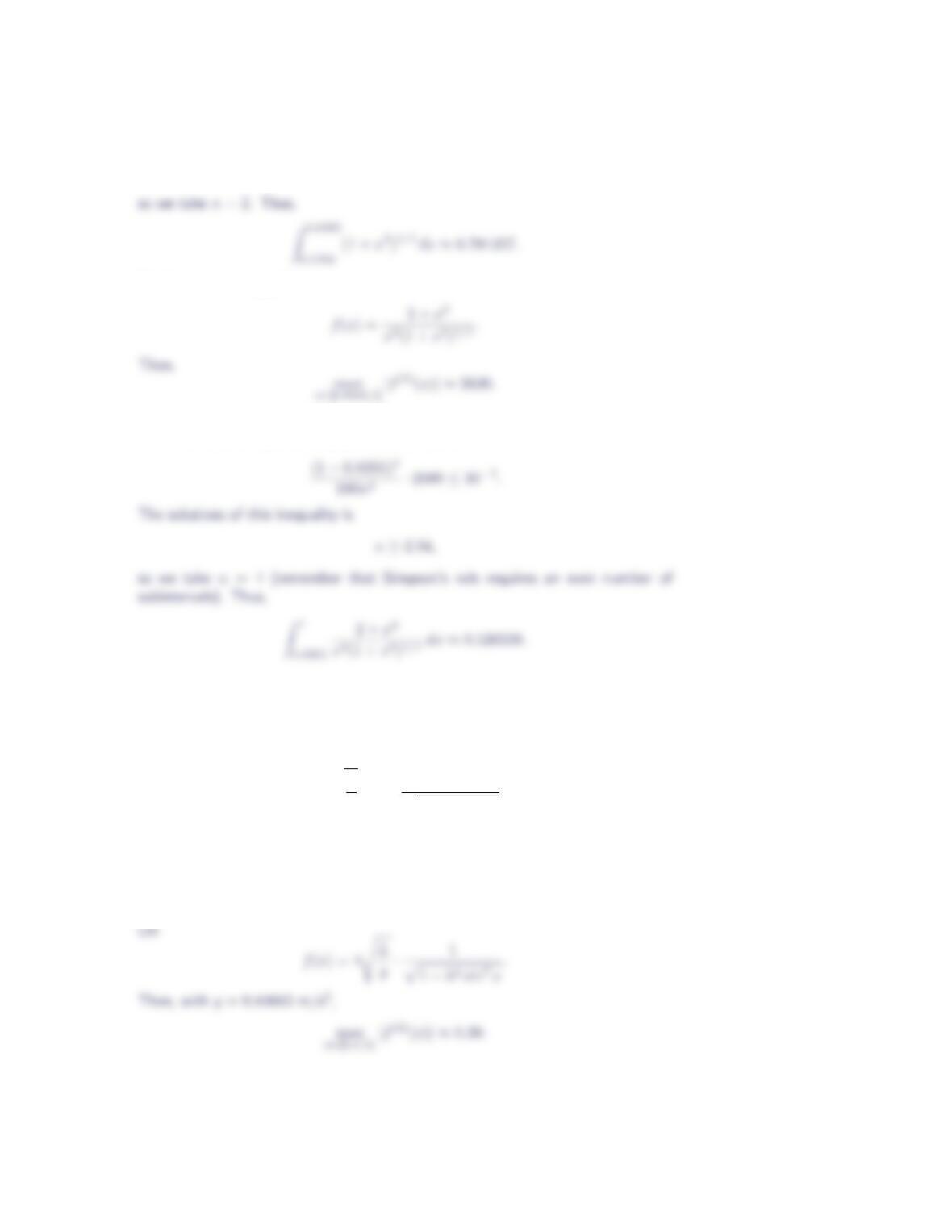
First, let
Then,
Composite Newton-Cotes Quadrature 21
For the second integral, let
The number of subintervals needed to guarantee an absolute error not greater than
10−4from the composite Simpson’s rule satisfies
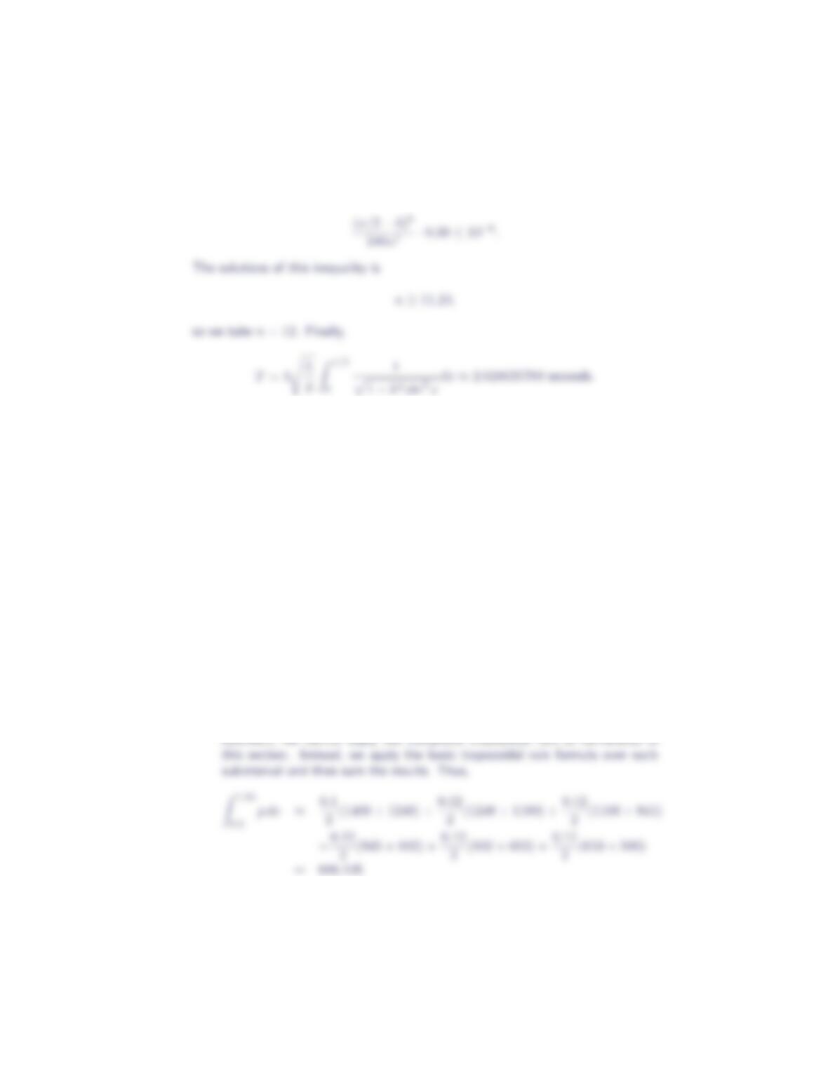
26. Using Newton’s Second Law, it can be shown that the period, T(the time
for one complete swing), of a pendulum with length Land maximum angle of
deflection θ0is given by
T= 4sL
gZπ/2
0
1
p1−k2sin2xdx,
where k= sin(θ0) and gis the acceleration due to gravity. To calibrate the tim-
ing mechanism in their top-of-the-line model, a grandfather clock manufacturer
needs to know the period of a pendulum with L= 1 meter and θ0= 12◦to
within 10−6seconds. Calculate the period to the required accuracy.
22 Section 6.5
The number of subintervals needed to guarantee an absolute error not greater than
10−6from the composite Simpson’s rule satisfies
27. Ammonia vapor is compressed inside a cylinder by an external force acting on
the piston. The following data give the volume, v, measured in liters, and the
pressure, p, measured in kilopascals.
v0.50 0.60 0.72 0.84 0.96 1.08 1.25
p1400 1248 1100 945 802 653 500
The work for the process is given by the integral
Z1.25
0.5
p dv.
Estimate the work done in the following ways:
(a) using the trapezoidal rule;
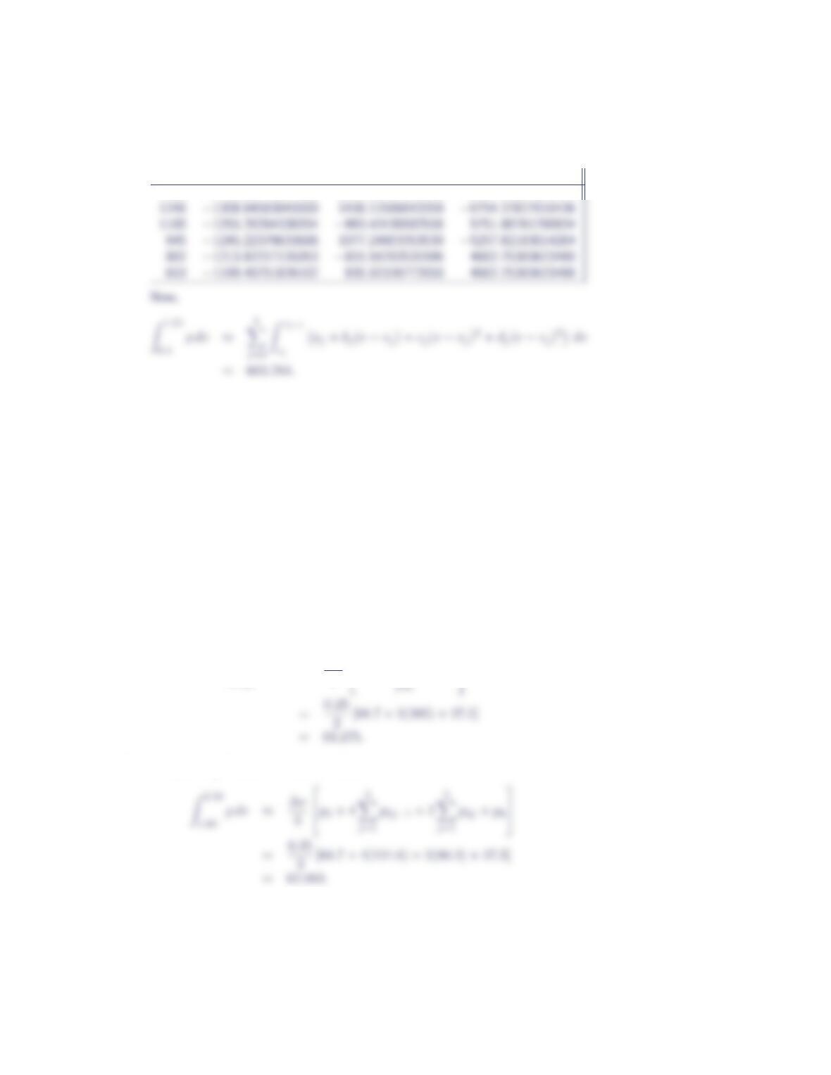
(b) by passing a cubic spline through the data and then integrating the spline.
(a) Because the change in vdoes not remain constant from measurement to mea-
(b) The coefficients of the not-a-knot cubic spline are
Composite Newton-Cotes Quadrature 23
ajbjcjdj
1400 −1798.89715224665 3464.39934948290 −6754.27827016436
28. Values of the volume (v, measured in cubic inches) and the pressure (p, measured
in pounds per square inch) of a gas as it expands from a volume of 1 cubic inch
to a volume of 2.5 cubic inches are presented in the table below.
v1.00 1.25 1.50 1.75 2.00 2.25 2.50
p68.7 55.0 45.8 39.3 34.4 30.5 27.5
The work done by the gas as it expands is given by
W=Z2.50
1.00
p dv.
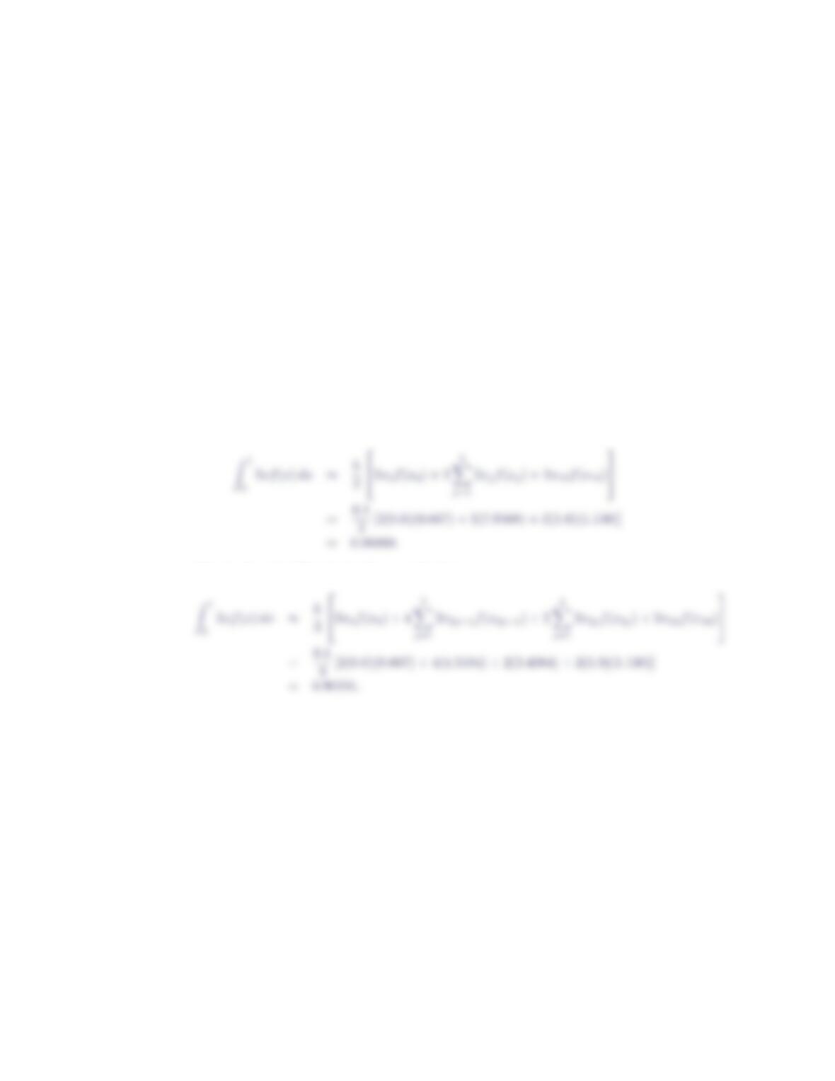
Estimate the value of this integral.
Using the trapezoidal rule, we calculate
Z2.50
1.00
p dv ≈∆v
2
p0+ 2
5
X
pj+p6
Alternately, using Simpson’s rule, we calculate
24 Section 6.5
29. Approximate the value of the integral
Z1
0
2xf(x)dx,
where fis given by
x0.0 0.1 0.2 0.3 0.4 0.5 0.6 0.7 0.8 0.9 1.0
f(x) 0.667 0.671 0.689 0.711 0.742 0.790 0.841 0.910 0.975 1.052 1.130
This integral arises in computing the mean flight distance of birds, randomly
dispersed throughout a circular region, to all other points of the region (see
J.F. Wittenberger and M.B. Dollinger, “The Effect of Acentric Colony Location
on the Energetics of Avian Coloniality,” American Naturalist, 124, 189 – 204,
1984).
Using the trapezoidal rule, we calculate
Alternately, using Simpson’s rule, we calculate