
Two types of demand relationships are stressed in the problems to Chapter 6: cross-price effects
and composite commodity results. The general goal of these problems is to illustrate how the
demand for one particular good is affected by economic changes that directly affect some other
portion of the budget constraint. Several examples are introduced to show situations in which the
analysis of such cross-effects is manageable.
Comments on Problems
6.1 Another use of the Cobb–Douglas utility function that shows that cross-price effects are
zero. Explaining why they are zero helps to illustrate the substitution and income effects
that arise in such situations.
6.2 Shows how some information about cross-price effects can be derived from studying
budget constraints alone. In this case, Giffen’s paradox implies that spending on all other
goods must decline when the price of a Giffen good rises.
6.3 A simple case of how goods consumed in fixed proportion can be treated as a single
commodity (buttered toast).
6.4 An illustration of the composite commodity theorem. Use of the Cobb–Douglas utility
produces quite simple results.
6.5 An examination of how the composite commodity theorem can be used to study the
effects of transportation or other transactions charges. The analysis here is fairly
intuitive—for more detail consult the Borcherding–Silverberg reference or Problem 6.12.
6.6 Illustrations of some of the applications of the results of Problem 6.5. More extensive
answers are provided in the solutions to Problem 6.12.
6.7 This problem demonstrates a special case in which uncompensated cross-price effects are
symmetric.
6.8 This problem looks at cross-substitution effects in a three-good CES function.
CHAPTER 6:
Demand Relationships among Goods

Chapter 6: Demand Relationships among Goods
46
Analytical Problems
6.9 Consumer surplus with many goods. This illustrates how expenditure functions can
help to clarify consumer surplus ideas when several prices change.
6.10 Separable utility. This problem shows that many of the complications in a many good
utility function can be greatly simplified if utility is assumed to be separable.
6.11 Graphing complements. The problem draws on Samuelson’s famous paper on
complementarity. It shows that there is a graphical representation of complements in the
three-good case that accurately reflects the Hicks definition.
6.12 Shipping the good apples out. This repeats the analysis in the Borcherding–Silberberg
paper in a simplified form. It is mainly intended to show how the various properties of
utility and demand function can be used to sign derivatives in special cases.
6.13 Proof of the composite commodity theorem. This problem outlines two general
approaches to proving the composite commodity theorem. The first, using duality, is
probably the most preferred such method.
6.14 Spurious product differentiation. This behavioral problem shows how firms may be
able to receive higher prices for their products if they can convince (spuriously)
consumers that they are better.
Solutions
6.1 a. As for all Cobb–Douglas applications, first-order conditions show
c. We have the two conditions
Chapter 6: Demand Relationships among Goods
47
d. From part (a),
6.4 a. The amount spent on ground transportation is
b. Maximize
Chapter 6: Demand Relationships among Goods
48
c. Although it might seem like increases in
t
would reduce expenditures on the
6.6 a. Transport charges make low-quality produce relatively more expensive at distant
6.7 Assume
ii
x a I=
and
.
jj
x a I=
Hence,
6.8 a. Example 6.3 gives
Chapter 6: Demand Relationships among Goods
49
b. The Slutsky equation shows
Analytical Problems
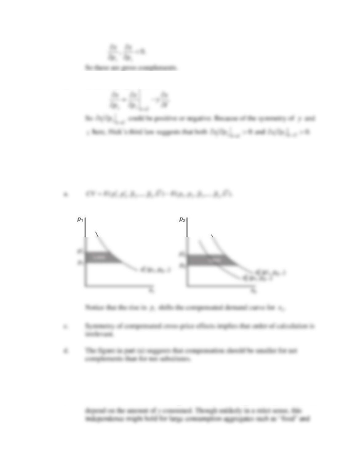
6.9 Consumer surplus with many goods
b.
c. Symmetry of compensated cross-price effects implies that order of calculation is
6.10 Separable utility
a. This functional form assumes
0.
xy
U=
That is, the marginal utility of
x
does not
Chapter 6: Demand Relationships among Goods
50
b. Because utility maximization requires
,
x x y y
MU p MU p=
an increase in
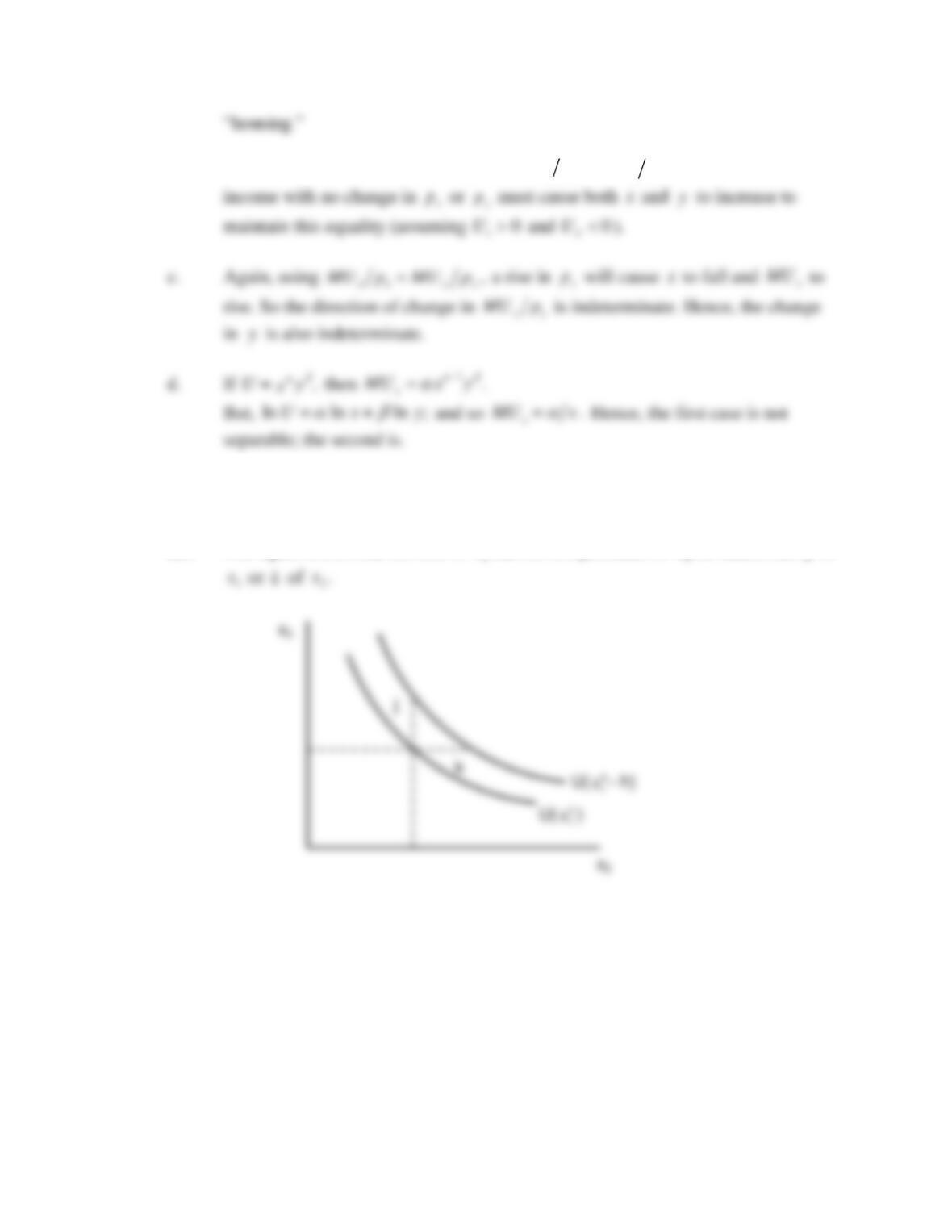
6.11 Graphing complements
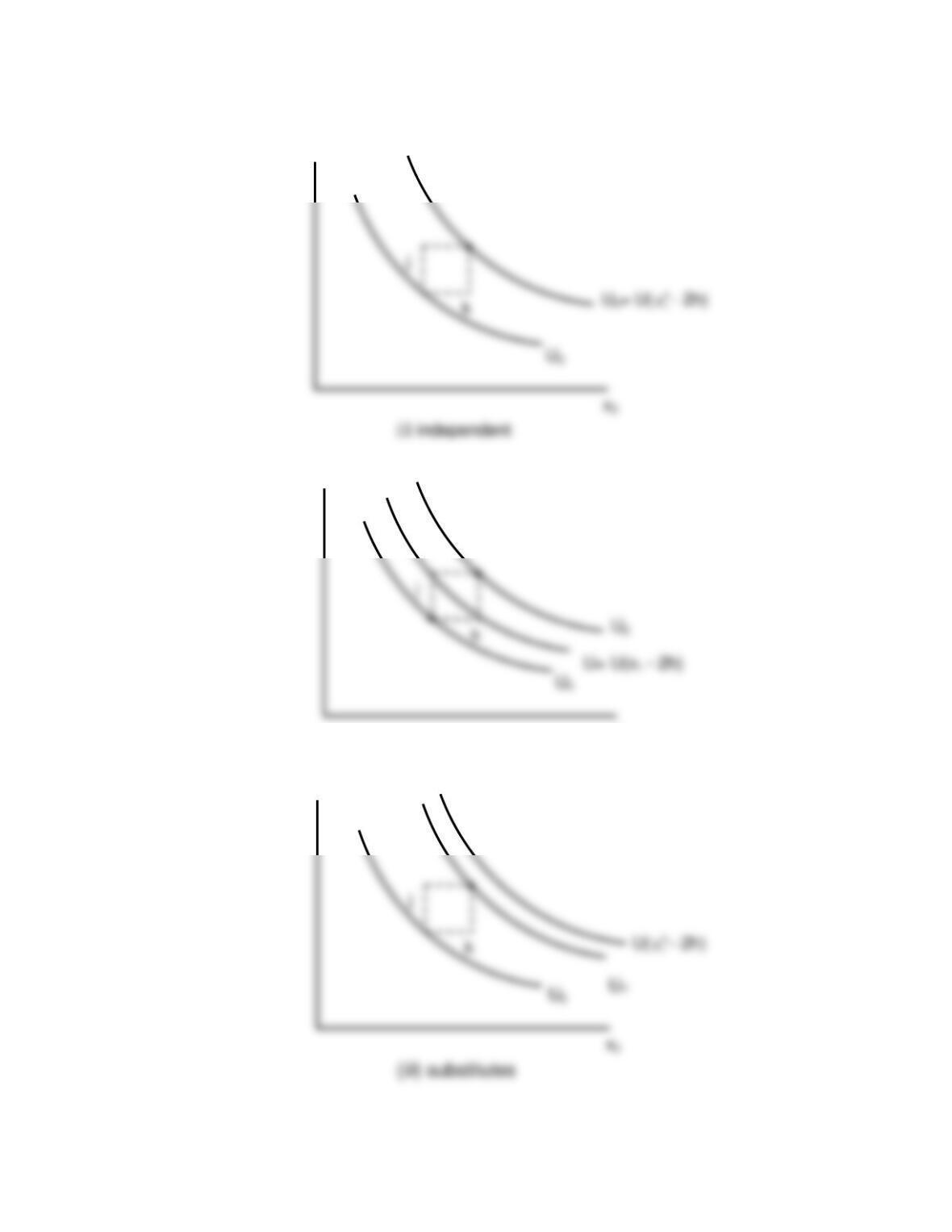
a,b. The figure shows that the loss in
x
can be compensated for by an additional
j
of
c. The new indifference curve is given by
2.U

Chapter 6: Demand Relationships among Goods
51
x3
U2
U0
x2
Chapter 6: Demand Relationships among Goods
52
d. The three cases are shown in the next three graphs:
U0
x2
(i) independent
x3
U2
U0
x3
x2
(ii) complements
x3
U0
x2
Chapter 6: Demand Relationships among Goods
53
e. Samuelson suggests the following proof. Consider the implicit equation:
This is the negative of the MRS. The MRS will remain constant since
1
p
and
2
p
remain constant. We wish to know how a change in
3
x
3
x
x
will change the levels of
f. The mathematical ideas will always be relevant since they are in principle
6.12 Shipping the good apples out
Chapter 6: Demand Relationships among Goods
54
c. Given
d. Hicks’ third law is
3
10
ij
je
==
, for
1,2,3.i=
If we substitute for
23
e
and
33
e
in
e. The own-price elasticity of
2,x
22 ,e
is negative. If goods 2 and 3 are substitutes,
Chapter 6: Demand Relationships among Goods
55
This term is likely to be small if we assume that goods 2 and 3 have similar
relationships with 1: that is,
31
e
and
21
e
31
e
21
e
should have close values. Since goods 2
and 3 are close substitutes, such an assumption seems reasonable. Therefore,
overall, we can expect the expression to be positive.
f. a) In this example, high-quality apples and fresh oranges can
be represented as good 2 (using the above notation) and the low-quality
b) In this example, expensive restaurant meals and cheap restaurant
c) We can assume that flying the Concorde falls in the category of expensive
flights, and these are close substitutes to cheaper flights. Thus, the
Chapter 6: Demand Relationships among Goods
56
d) In this example, the value of the time spent searching is a transaction cost
6.13 Proof of the composite commodity theorem
a. Proof using duality
i. Applying the envelope theorem to both minimization problems yields:
b. Proof using two-stage maximization
i. Because neither the price of
23
or xx
changes, the maximum value for the
ii. This equality is derived by repeated application of the envelope theorem to the

Chapter 6: Demand Relationships among Goods
57
6.14 Spurious product differentiation
a. The first-order condition for utility maximization for brand 1 is
11
500 (1 )
y
py=+
.
d.Spending funds to ascertain the quality of brand 2 (say by reading Consumer Reports)
would be equivalent to taking a gamble whose outcome depends on whether the