Also, 2
12
3
lb
0.167 lb
ft 0.334 ft
6in.
in.
12 ft
pp
p
x
−
∂
−= = =
∂
thus, from Eq. (1)
Problem 6.83
A flat block is pulled along a horizontal flat surface by a horizontal rope perpendicular to
one of the sides. The block measures
1.0 m 1.0 m×, has a mass of
1
00 kg and a constant ve-
locity of m
1
.0 s, and is separated from the flat surface by a 0.1-cm-thick oil layer of 15 °C
SAE 20 crankcase oil. Find the coefficient of sliding friction for the block. Does this coeffi-
cient of friction change with the velocity?
Solution 6.83
The force resisting the block’s motion is
F
A
τ
=.
Since the gap is thin, assume that the velocity profits in the oil is linear so
Problem 6.84
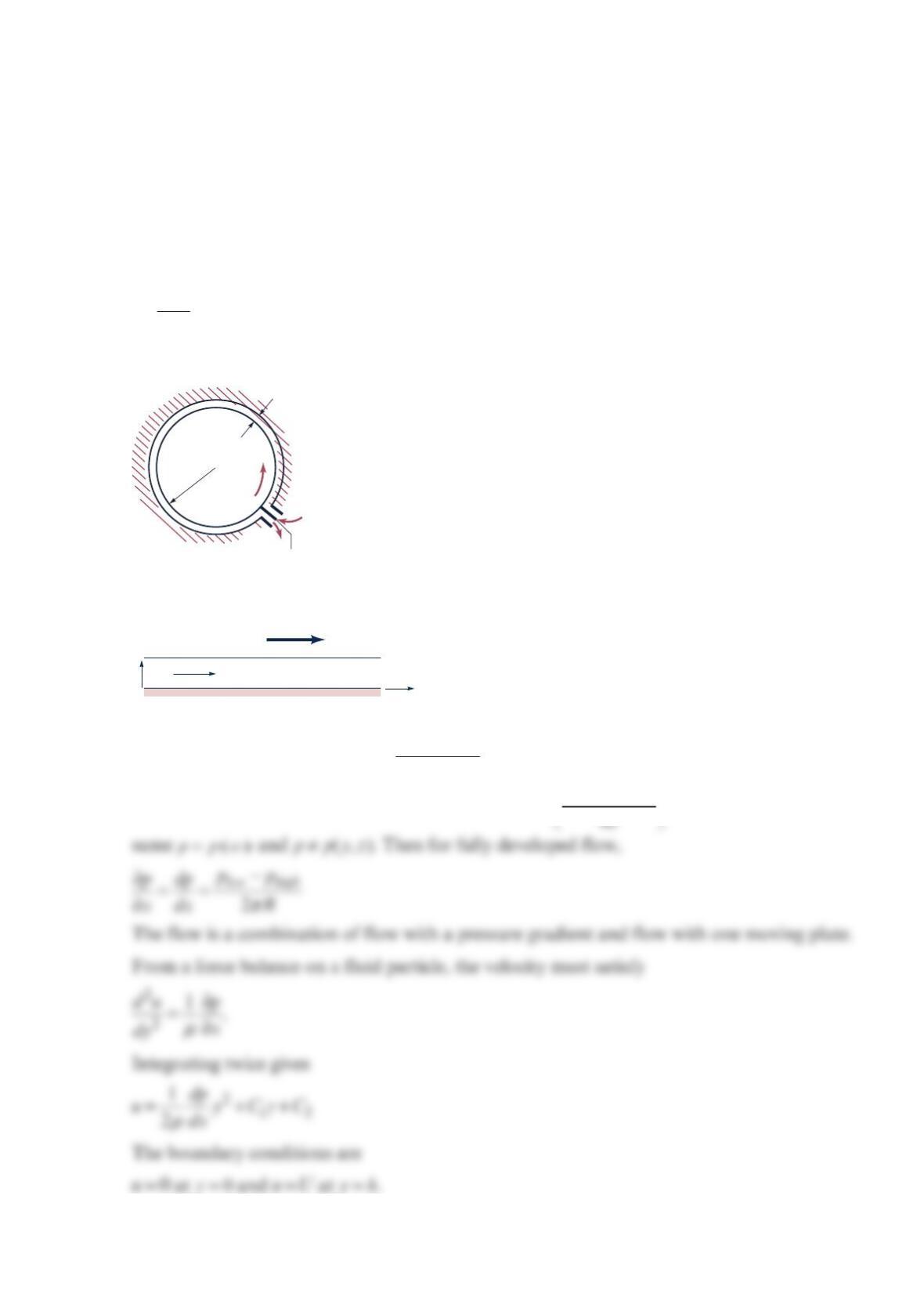
A viscosity motor/pump is shown in the figure below. The rotor is concentric within a sta-
tionary housing. The clearance h between the housing and the rotor is small compared to
the width
w
and radius
R
of the rotor. A seal divides the clearance space as shown.When
the device is operated as a motor, the viscous liquid is introduced at the high-pressure side
of the seal and leaves at the low-pressureside of the seal. This flow causes the rotor to turn
and produce power. For 1.0 f
t
R
=, 0.50 in.h=, 1.0 ftw=, 10 rpm
ω
=, and a flowrate of
3
ft
1
.5 min, find the power output of the rotor.The fluid is 60 °F, SAE 30 crankcase oil. Ne-
glect gravity.
Solution 6.84
Since h
R
<< , we can neglect the curvature and model the flow as that between parallel
plates with fully developed flow ()
0
velocity
x
∂
=
∂
. We will assume the two plates are infi-
nitely wide so there is no variations in the z direction ()
0
anything
∂
=
Seal (no drag on rotor)
p
low
p
high
h
Rotor
+
Housing
R
ω
yq
x
u
=
R
ω
Solving for 1
C
and 2
C
, the velocity profile gives
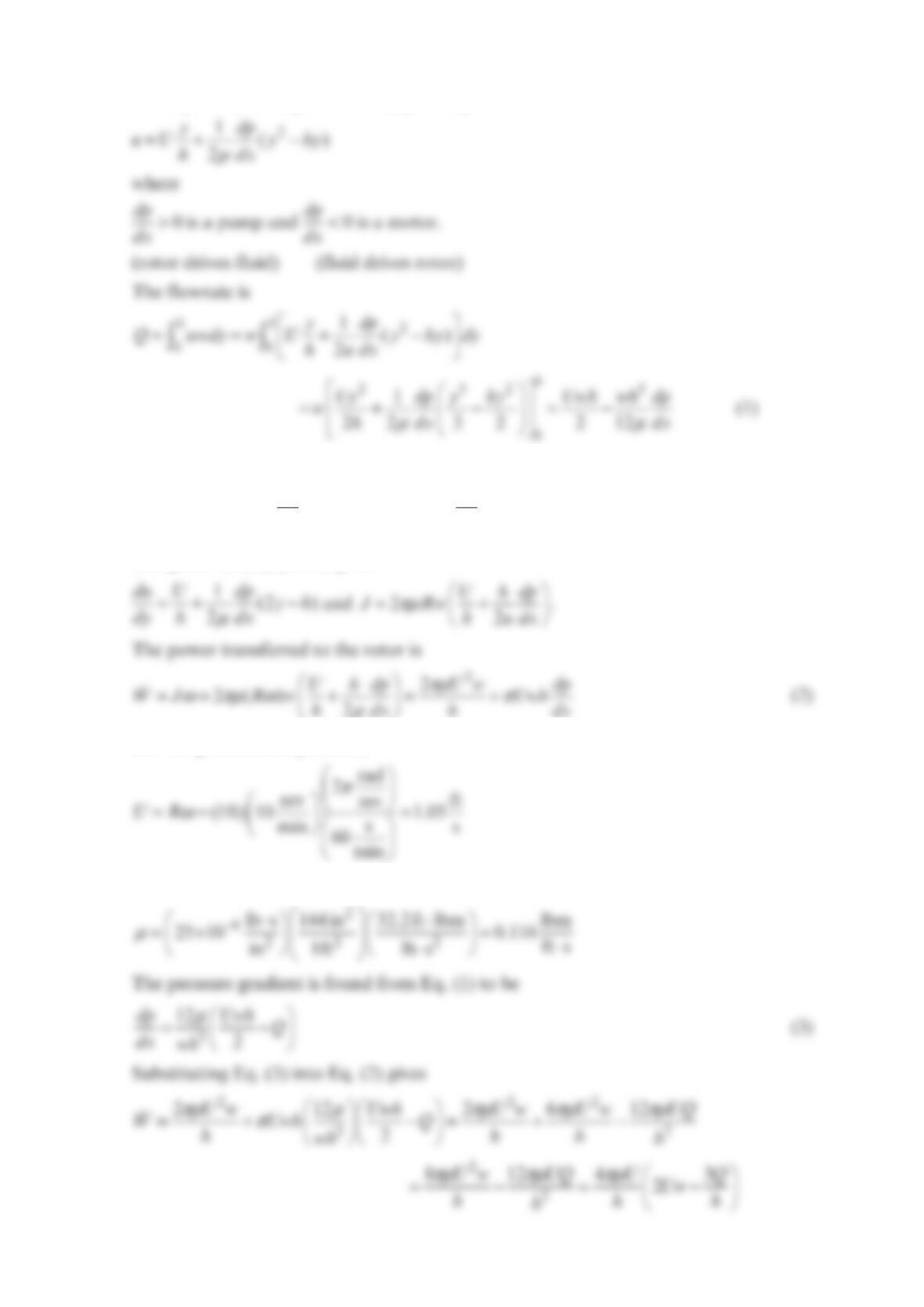
The torque on the rotor is due to shear stress
2
02
hyh
du du
J dA wRd Rw
dy dy
π
τµθπµ
=
== =
.
Using the velocity profile gives
(2)
For the given motor problem,
Figure A.2 gives
The numerical values give
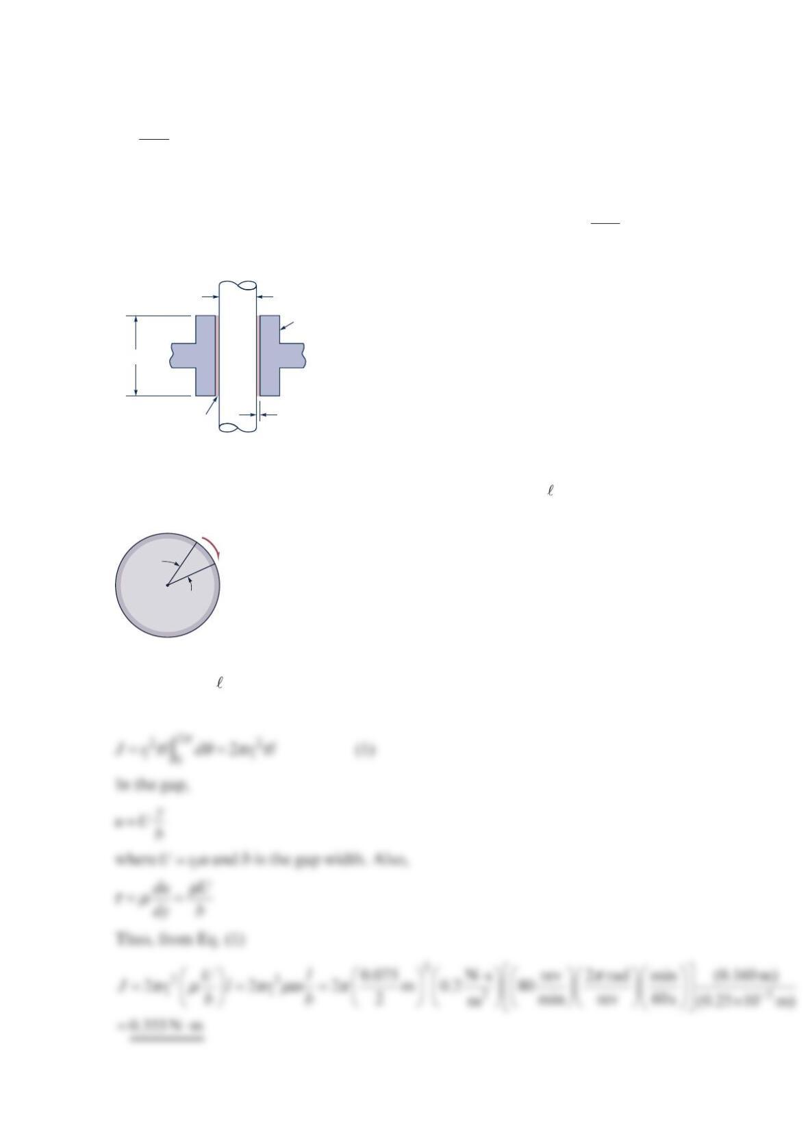
Problem 6.85
A vertical shaft passes through a bearing and is lubricated with an oil having a viscosity of
2
Ns
0.2 m
⋅ as shown in the figure below. Assume that the flow characteristics in the gap
between the shaft and bearing are the same as those for laminar flow between infinite
parallel plates with zero pressure gradient in the direction of flow. Estimate the torque re-
quired to overcome viscous resistance when the shaft is turning at rev
8
0min.
Solution 6.85
The torque due to force dF acting on a differential area, i
d
Ard
θ
=, is (see in the figure be-
low)
2
ii
d
JrdFr d
τ
θ
==
where
τ
is the shearing stress. Thus,
0.25 mm
75 mm
Shaft
Oil
160 mm
Bearing
ℓ
~ shaft length
ℓ
dF
=
dA
=
θ
d
θ
d
r
i
r
i
r
i
τ
τ
ω
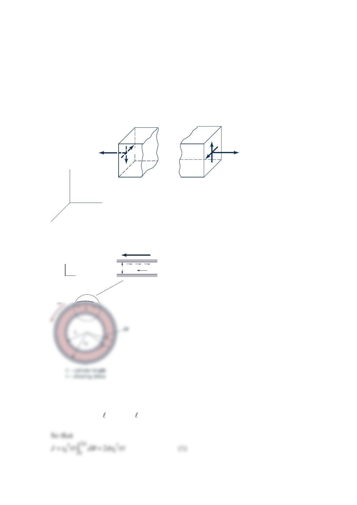
Problem 6.86
A viscous fluid is contained between two long concentric cylinders. The geometry of the
system is such that the flow between the cylinders is approximately the same as the laminar
flow between two infinite parallel plates. (a) Determine an expression for the torque re-
quired to rotate the outer cylinder with an angular velocity
ω
. The inner cylinder is fixed.
Express your answer in terms of the geometry of the system, the viscosity of the fluid,
and the angular velocity. (b) For a small, rectangular element located at the fixed wall,
determine an expression for the rate of angular deformation of this element. (See the
figure below.)
Solution 6.86
(a) The torque which must be applied to outer cylinder to overcome the force due to the
shearing stress is (see the figure above)
2
000 0
()
d
JrdFrrd r d
τθ τ
θ
== =
z
x
y
(
b
)(
a
)
A’ A
C’ C
B
B’
D’ D
xx
xy
xz xx
xy
xz
τ
σσ τ
τ
τ
y
x
r0 – ri = b
τ
u
U = r0
ω
(b) From the equation
vu
xy
γ
∂∂
=+
∂∂
For the linear distribution
0
0i
rUy
uy
rr b
ω
=− =−
−
Problem 6.87
Verify that the momentum correction factor
β
for fully developed, laminar flow in a circu-
lar tube is 4
3.
Solution 6.87
The fully developed velocity profile for the axial velocity
u
is
where
V
is the average velocity defined by
Now
0
Then
Problem 6.88
Verify that the kinetic energy correction factor
α
for fully developed, laminar flow in a cir-
cular tube is 2.0.
Solution 6.88
The fully developed velocity profits for the axial velocity
u
is
2
max 2
1r
uu R
=−
.
Equation (7.42) gives
Now
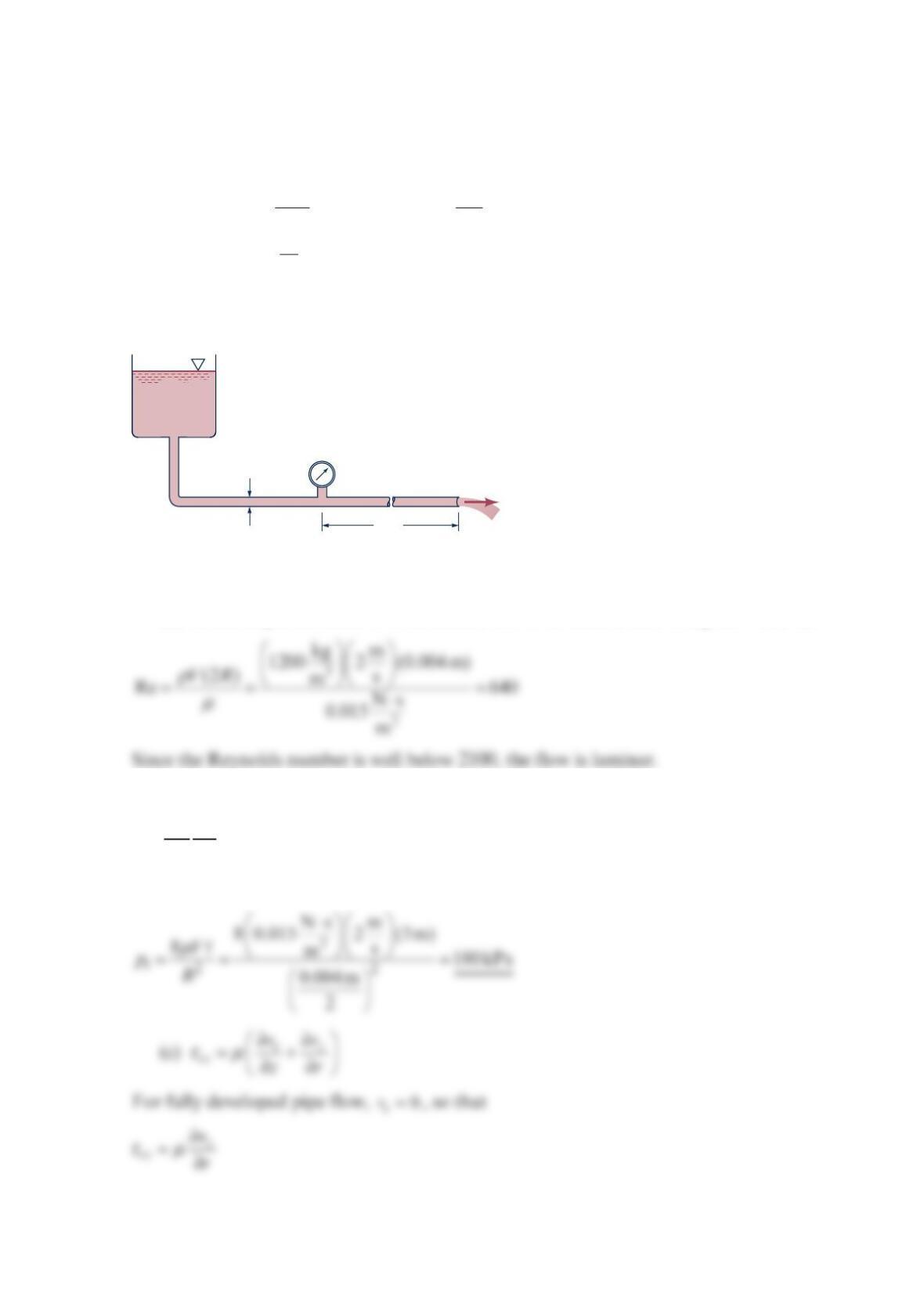
Problem 6.89
A simple flow system to be used for steady-flow tests consists of a constant head tank con-
nected to a length of 4-mm-diameter tubing as shown in the figure below. The liquid has a
viscosity of 2
Ns
0.015 m
⋅, a density of 3
kg
1
200 m, and discharges into the atmosphere with a
mean velocity of m
2
s. (a) Verify that the flow will be laminar. (b) The flow is fully devel-
oped in the last
3
m of the tube. What is the pressure at the pressure gage? (c) What is the
magnitude of the wall shearing stress, rz
τ
, in the fully developed region?
Solution 6.89
(a) Check Reynolds number to determine if flow is laminar (See Chapters 7 and 8):
(b) For laminar flow,
2
8
Rp
V
l
µ
Δ
=
Since 12 1
0
p
pp p
Δ
=− =−
(see the figure in the Problem)
Pressure
gage
3 m
Diameter = 4 mm
Also,
2
max 1
z
r
vv R
=−
2
Problem 6.90
(a) Show that for Poiseuille flow in a tube of radius
R
, the magnitude of the wall shearing
stress, rz
τ
, can be obtained from the relationship
3
4
()
rz wall
Q
R
µ
τπ
=
for a Newtonian fluid of viscosity
µ
. The volume rate of flow is
Q
. (b) Determine the mag-
nitude of the wall shearing stress for a fluid having a viscosity of 2
Ns
0.004 m
⋅ flowing with an
average velocity of mm
1
30 s in a 2-mm-diameter tube.
Solution 6.90
(a)
τµ
∂∂
=+
∂∂
rz
rz
vv
zr
For Poiseuille flow in a tube, 0
r
v=, and therefore
µ
Problem 6.91
An infinitely long, solid, vertical cylinder of radius
R
is located in an infinite mass of an in-
compressible fluid. Start with the Navier–Stokes equation in the
θ
direction and derive an
expression for the velocity distribution for the steady-flow case in which the cylinder is ro-
tating about a fixed axis with a constant angular velocity
ω
. You need not consider body
forces. Assume that the flow is axisymmetric and the fluid is at rest at infinity.
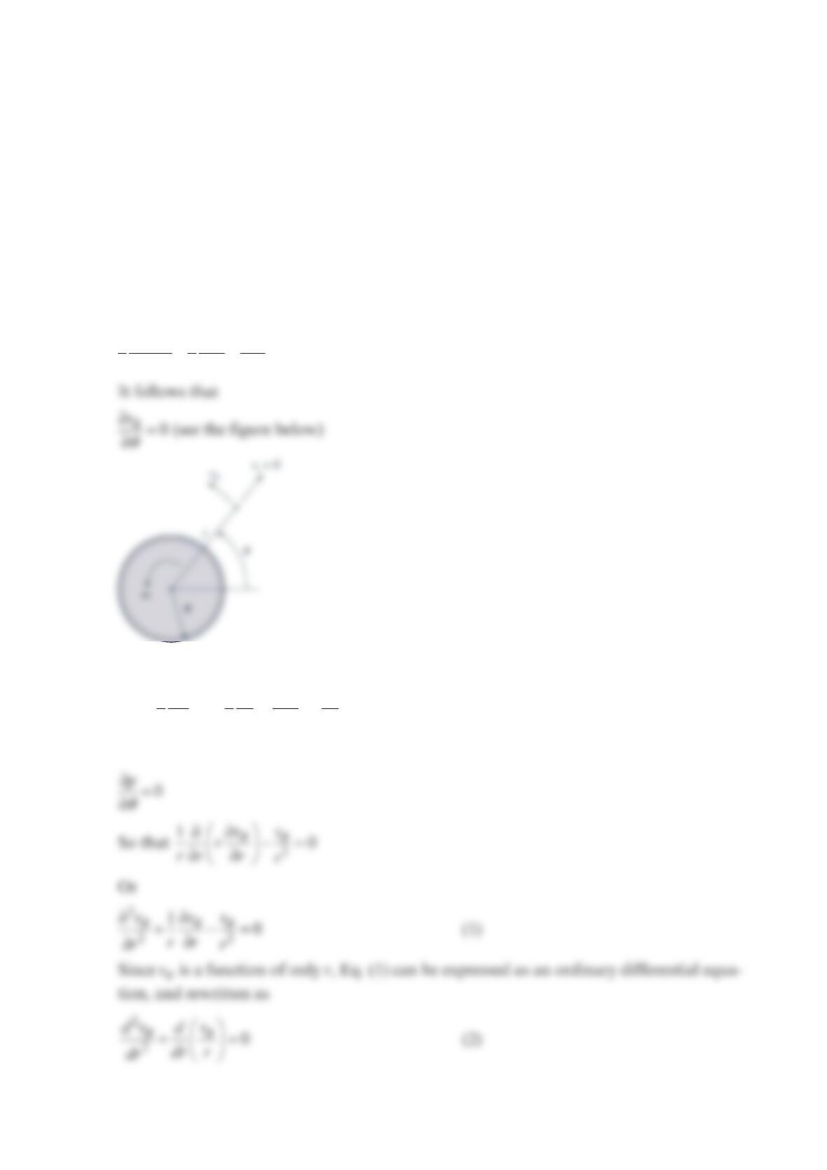
Solution 6.91
For this flow field, 0
r
v=, 0
z
v=, and from the continuity equation,
()
11 0
rz
v
rv v
rr r z
θ
θ
∂
∂∂
++=
∂∂∂
Thus, the Navier–Stokes equation in the
θ
-direction for steady flow reduces to
θθ
µ
θ
∂
∂∂
=− + −
∂∂∂
2
11
0vv
pr
rrrr
r
Due to the symmetry of the flow,
Equation (2) can be integrated to yield
1
dv v C
dr r
θθ
+=
Or
And a second integration yields
2
12
2
Cr
rv C
θ
=+
Or