Problem 5.19
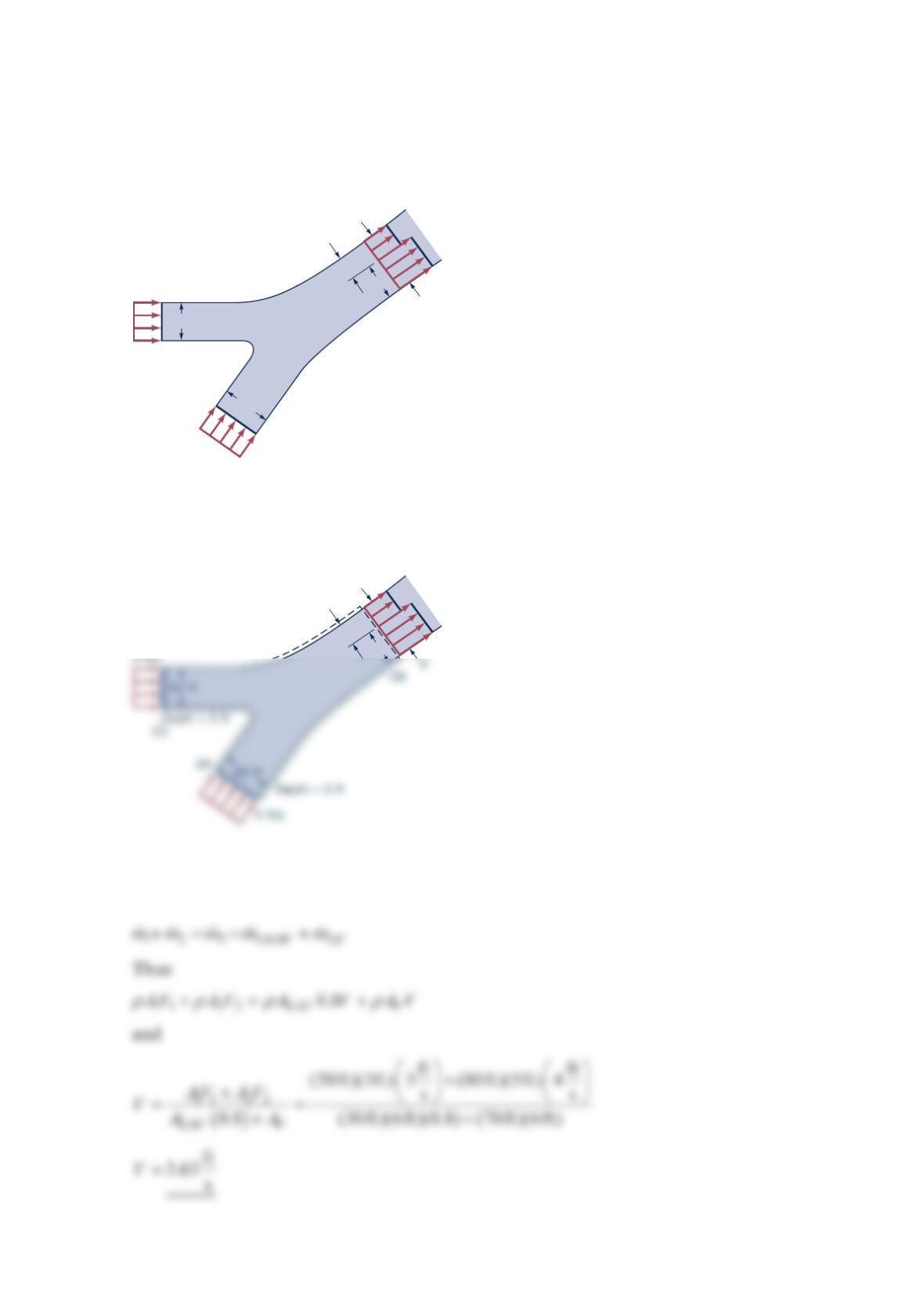
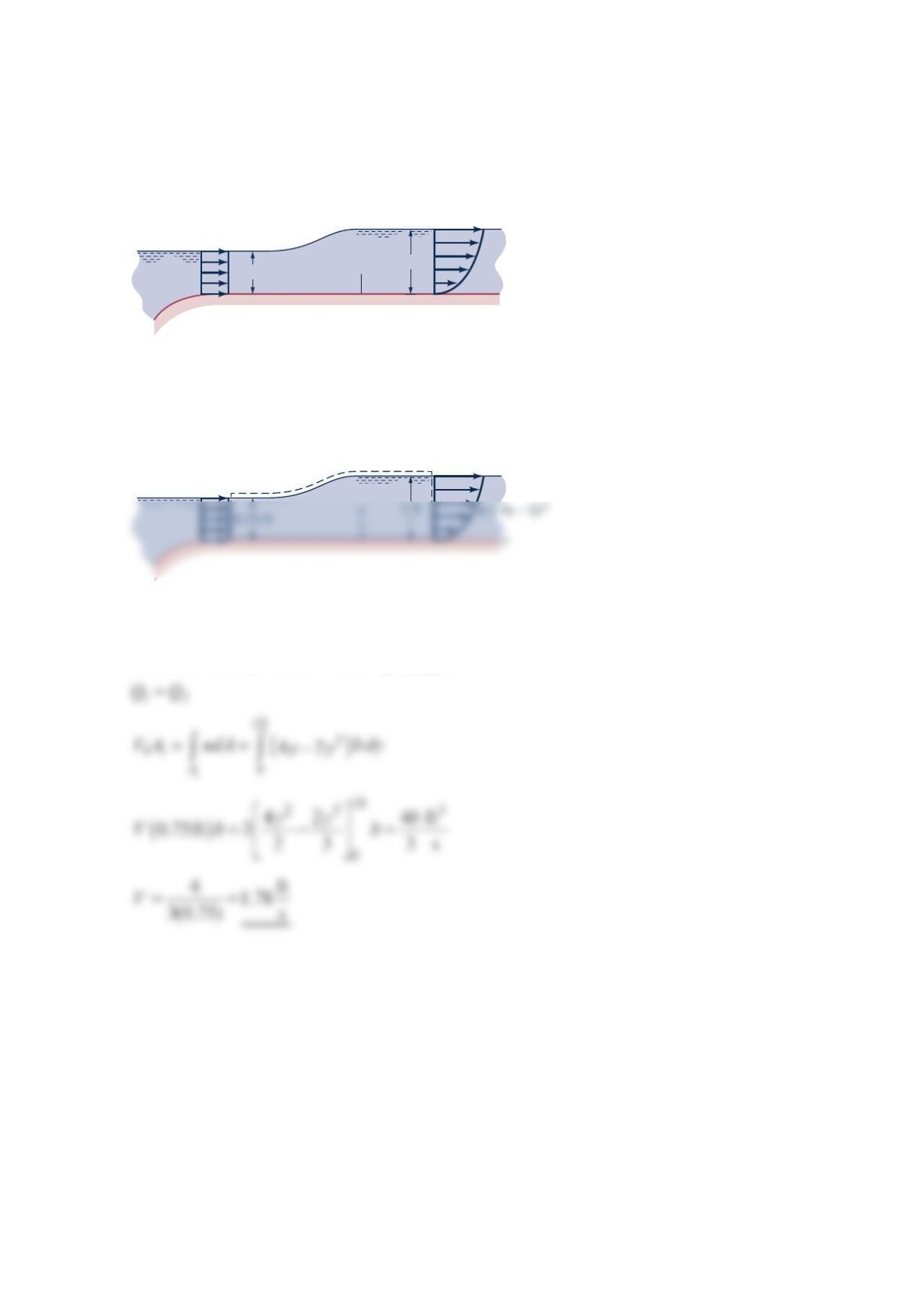
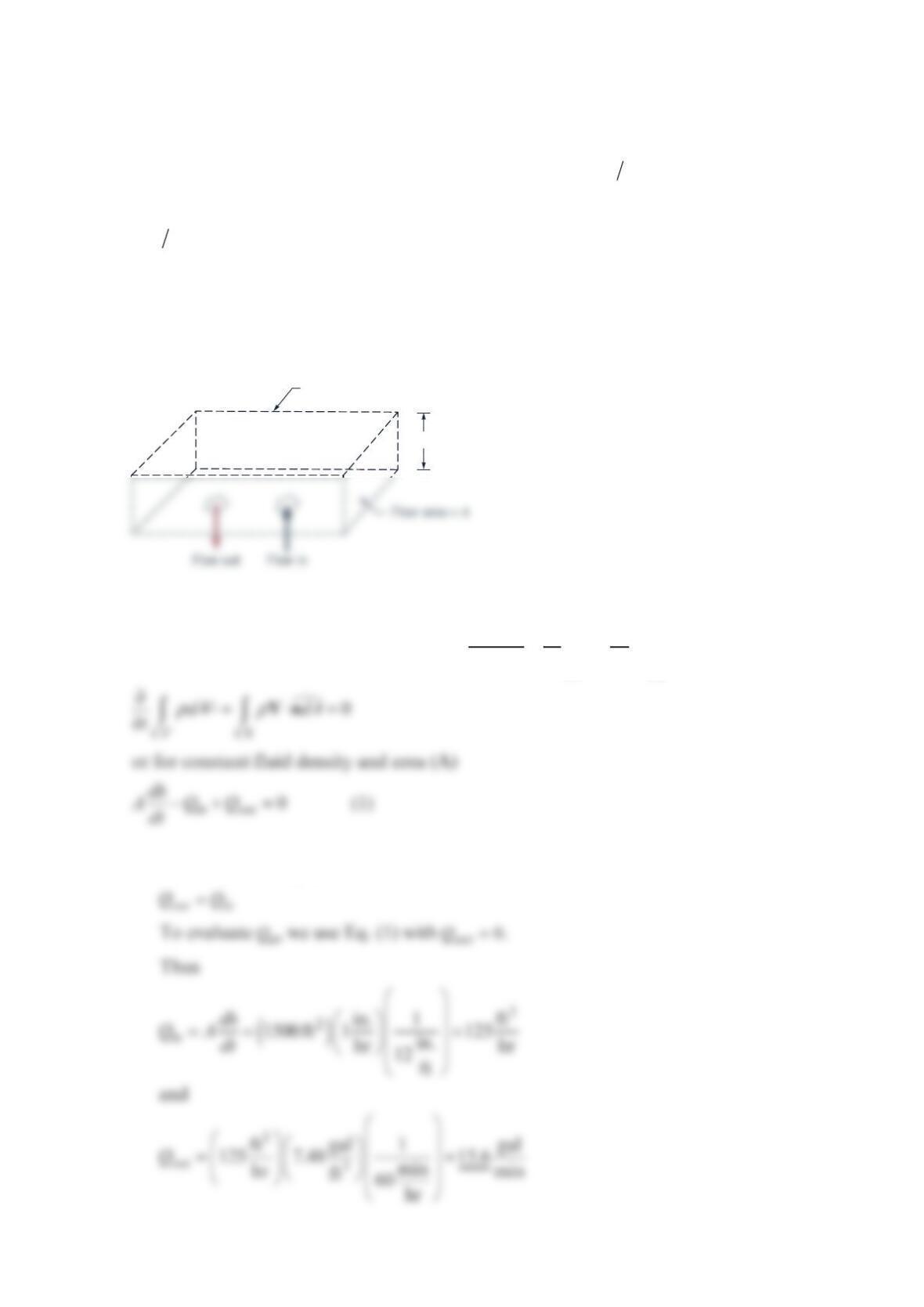
Two rivers merge to form a larger river as shown in the figure below. At a location
downstream from the junction (before the two streams completely merge), the nonuniform
velocity profile is as shown and the depth is 6ft. Determine the value of
V
.
Solution 5.19
Use the control volume shown within broken lines in the sketch above. We note that
mAV
ρ
=
and from the conservation of mass principle, we get
4 ft/s
3 ft/s
Depth = 3 ft
Depth = 5 ft
80 ft
50 ft
0.8
V
V
70 ft
30 ft
0.8 V
70 ft
30 ft
Problem 5.20
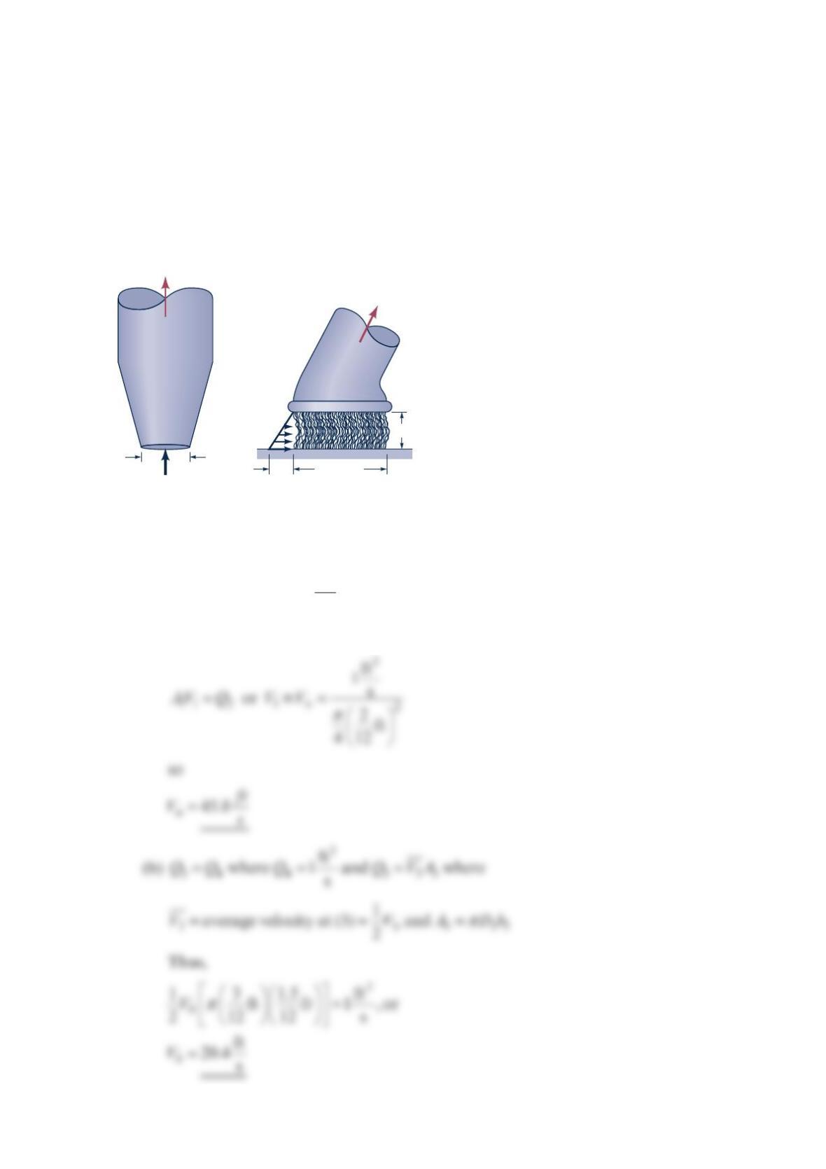
Various types of attachments can be used with a shop vac. Two such attachments are
shown in the figure below—a nozzle and a brush. The flowrate is 3
1ft /s . (a) Determine the
average velocity through the nozzle entrance, n
V
. (b) Assume the air enters the brush
attachment in a radial direction all around the brush with a velocity profile that varies
linearly from 0 to b
V
along the length of the bristles as shown in the figure. Determine the
value of b
V
.
Solution 5.20
(a) = =
3
12 2
ft
where 1 s
QQ Q
Thus,
Q
= 1 ft
3
/s
Q
= 1 ft
3
/s
Vn
2-in. dia.
1.5 in.
3-in. dia.
Vb
Problem 5.21
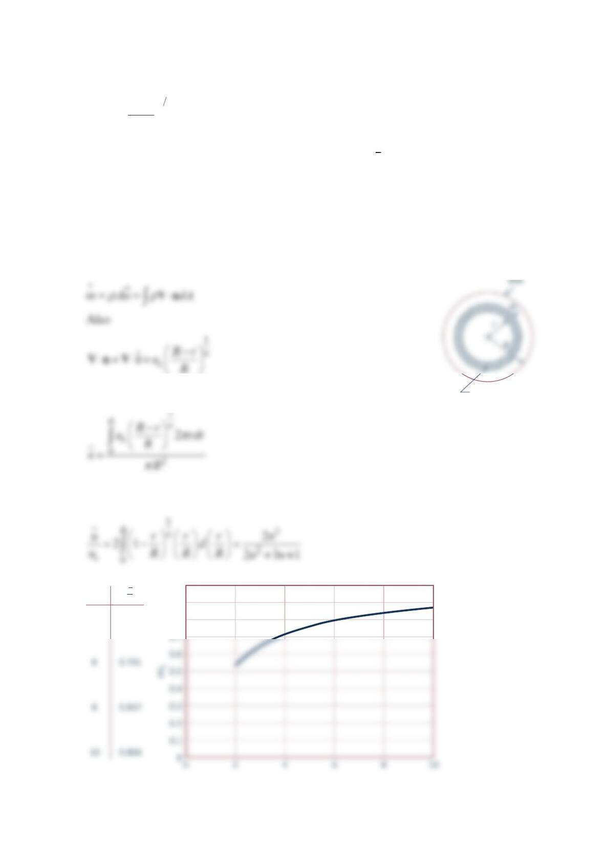
An appropriate turbulent pipe flow velocity profile is
−
=
1
c
n
Rr
uR
Vi
where c
u = centerline velocity,
r
= local radius,
R
= pipe radius, and i
= unit vector along
pipe centerline. Determine the ratio of average velocity, u, to centerline velocity, c
u, for (a)
n = 4, (b) n = 6, (c) n = 8, (d) n = 10. Compare the different velocity profiles.
Solution 5.21
For any cross section area
Thus for a uniformly distributed density,
ρ
, over area
A
and
1
0.9
0.8
4
n
0.711
u
u
c
Cross section
dA = 2
π
rdr
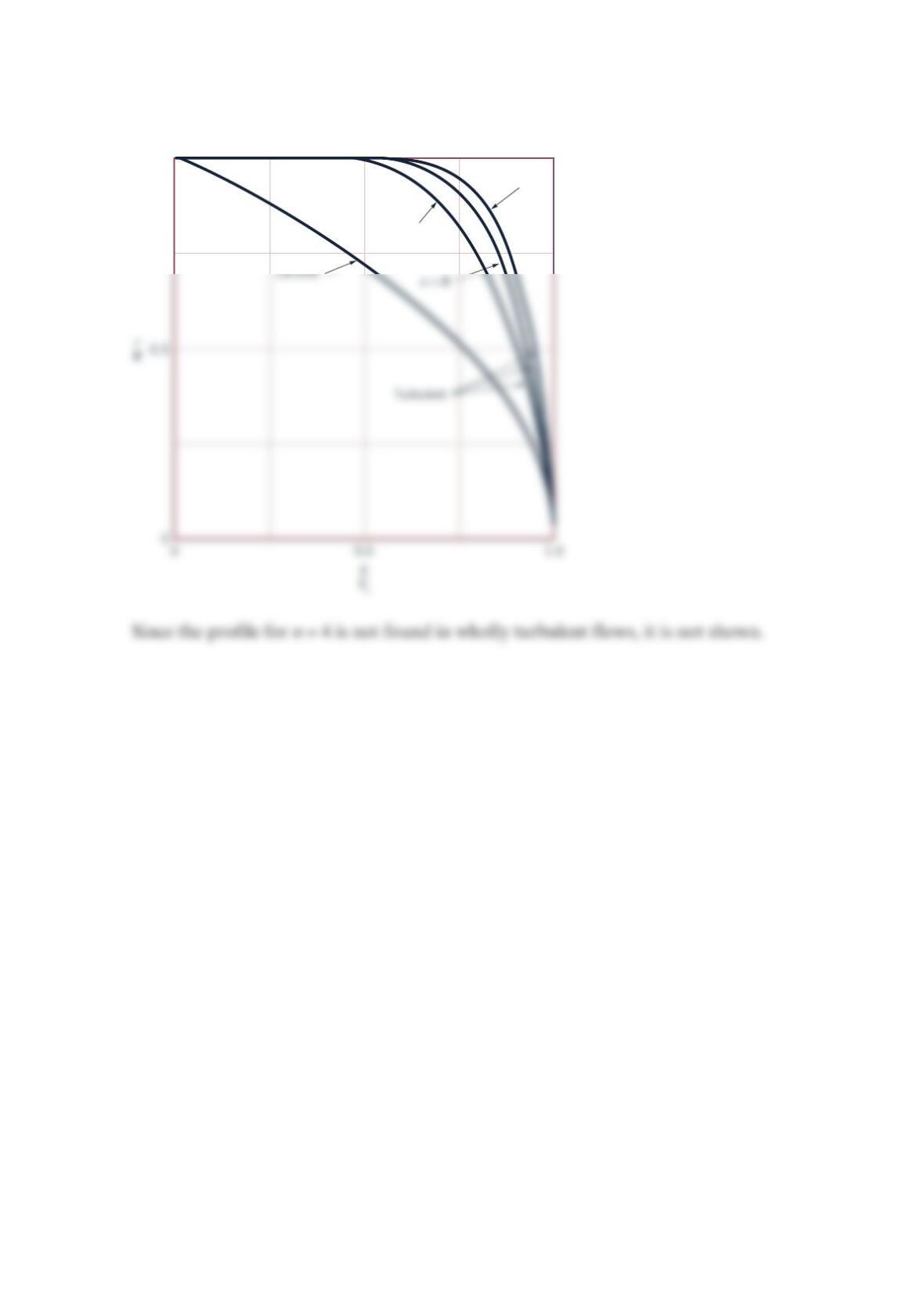
The different velocity profiles (including for laminar flow) are compared in the figure
below.
1.0
n
= 10
n
= 6
Problem 5.22
As shown in the figure below, at the entrance to a 3-ft-wide channel, the velocity
distribution is uniform with a velocity
V
. Further downstream, the velocity profile is given
by
2
42uyy=− , where u is in
f
t/s and y is in ft. Determine the value of
V
.
Solution 5.22
Use the control volume indicated by the broken lines in the sketch above.
From the conservation of mass principle
u
= 4
y
– 2
y
2
x
1 ft
0.75 ft
y
V
(1)
(2)
V
Problem 5.23
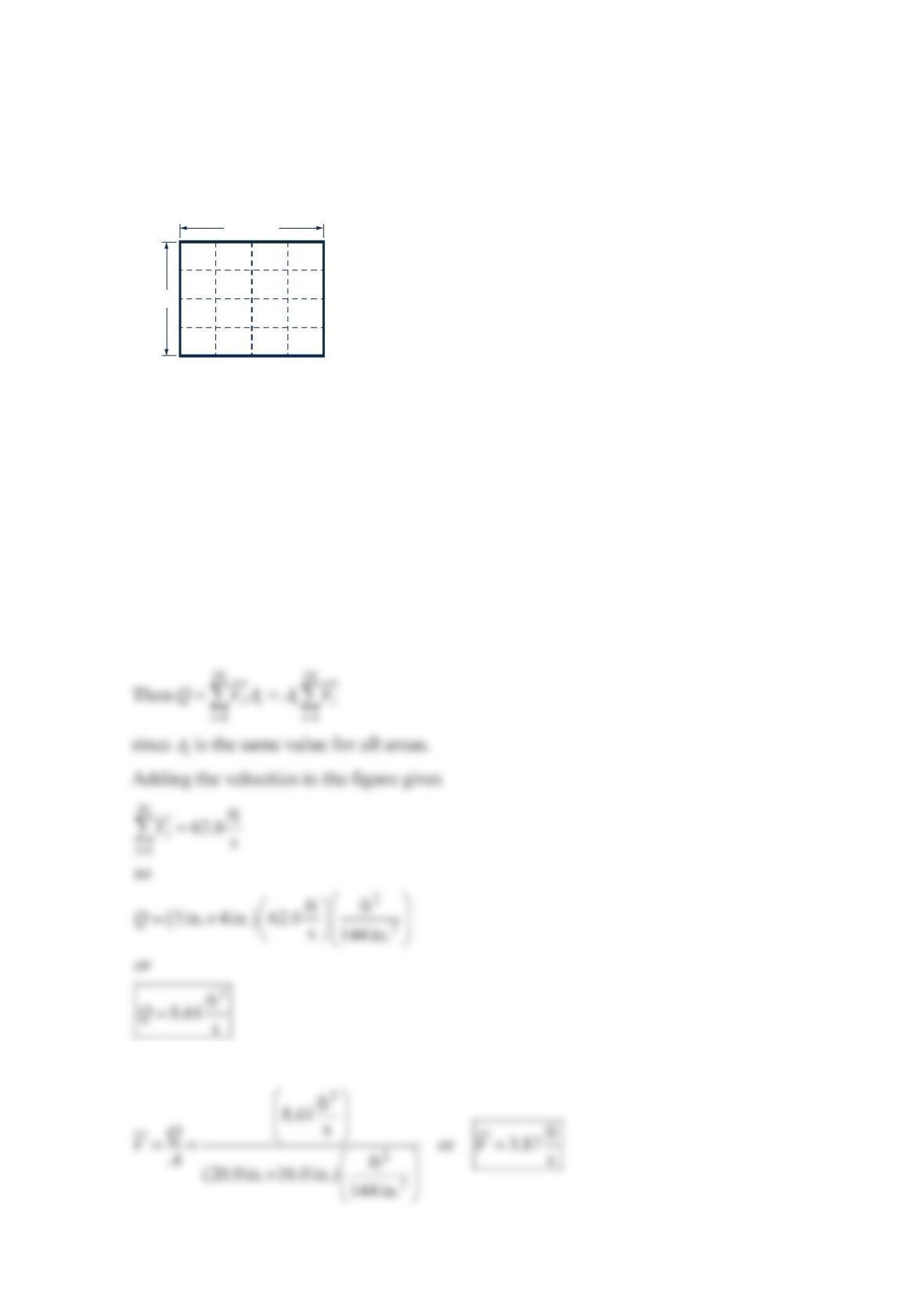
The cross-sectional area of a rectangular duct is divided into 16 equal rectangular areas, as
shown in the figure below. The axial fluid velocity measured in feet per second in each
smaller area is given in the figure. Estimate the volume flowrate and average axial velocity.
Solution 5.23
GIVEN: Axial velocities measured in rectangular duct shown in the figure in the problem.
FIND: Estimate volume flowrate and average velocity.
SOLUTION:
A
QdA=⋅
Vn
The velocity in each small rectangular area is assumed to be the average velocity for that
area.
The average velocity for the entire duet is
3.0 3.4 3.6
20.0 in.
Velocities in ft/s
16.0 in.
3.1
3.7 4.0 3.9 3.8
3.9 4.6 4.5 4.2
3.7 4.4 4.3 3.9
Problem 5.24
Oil for lubricating the thrust bearing shown in the figure below flows into the space
between the bearing surfaces through a circular inlet pipe with velocity
2
01r
uU R
=−
,
where 1.5 mm
R
=. The oil has a specific gravity SG = 0.86 and flows in the inlet pipe
at a rate of 0.006 kg/s. Compute the average velocity 1
V
of the oil in the inlet pipe and
the average velocity 2
V
at the outlet (plane 2) and the maximum velocity in the oil inlet
pipe ( 0
U
). Assume radial flow.
Solution 5.24
GIVEN: Inlet oil velocity =
2
01r
uU R
=−
, oil flowrate 0.006 kg/s, oil specific gravity =
SOLUTION: To find the average velocity 1
V
, we use the flowrate
Q
The velocity 2
V
is found from
D2 = 10 cm
D1 = 3.0 mm = 2R
u = U0 1 –
= oil velocity profile
Circular disc
(
(
r
R
r
h = 2.0 mm
Outlet
plane 2
Inlet
pipe 2
V
V
U
The velocity 0
U
is found by first finding the volume flowrate
So
Problem 5.25
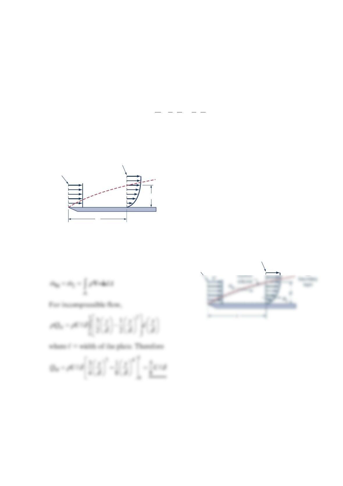
Flow of a viscous fluid over a flat plate surface results in the development of a region of
reduced velocity adjacent to the wetted surface as depicted in the figure below. This region
of reduced flow is called a boundary layer. At the leading edge of the plate, the velocity
profile may be considered uniformly distributed with a value
U
. All along the outer edge of
the boundary layer, the fluid velocity component parallel to the plate surface is also
U
. If
the x-direction velocity profile at section (2) is
3
31
22
uy y
U
δδ
=−
develop an expression for the volume flowrate through the edge of the boundary layer from
the leading edge to a location downstream at x where the boundary layer thickness is
δ
.
Solution 5.25
Consider the control volume shown. Apply
the Conservation of Mass principle to get
U
U
x
Section (1)
Section (2)
Outer edge
of
boundary
layer
δ
U
Section (1)
Section (2)
Outer edge
of
Problem 5.26
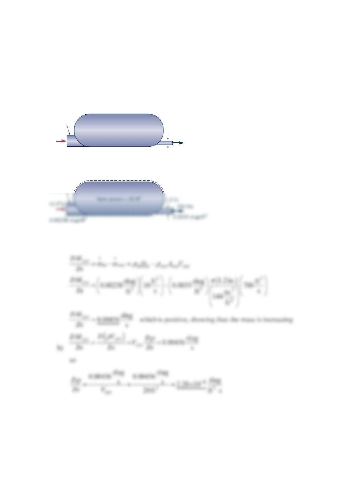
Air at standard conditions enters the compressor shown in the figure below at a rate of
3
10 ft /s . It leaves the tank through a 1.2-in.-diameter pipe with a density of 3
0.0035slugs/ft
and a uniform speed of 700 ft/s . (a) Determine the rate (slugs/s) at which the mass of air in
the tank is increasing or decreasing. (b) Determine the average time rate of change of air
density within the tank.
Solution 5.26
Use the control volume within the broken lines.
(a) From the conservation of mass principle, we get
Tank volume = 20 ft
3
1.2 in.
700 ft/s
0.0035 slugs/ft
3
10 ft
3
/s
Compressor
0.00238 slugs/ft
3
Compressor
Problem 5.27
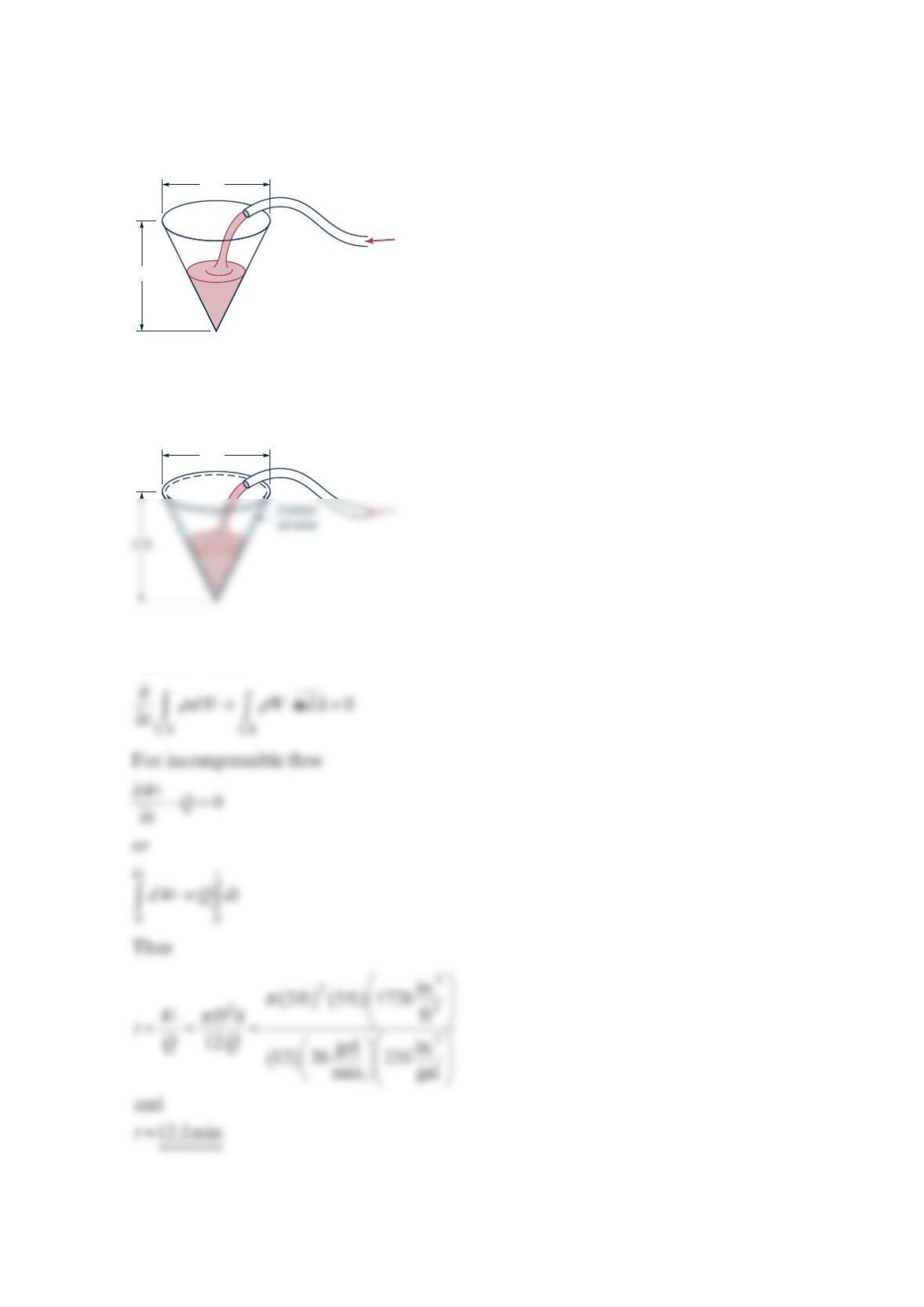
Estimate the time required to fill water in a cone-shaped container (see the figure below)
5ft high and 5ft across at the top if the filling rate is 20 gal/min.
Solution 5.27
From application of the conservation of mass principle to the control volume shown in the
figure, we have
5 ft
5 ft
5 ft
Problem 5.29
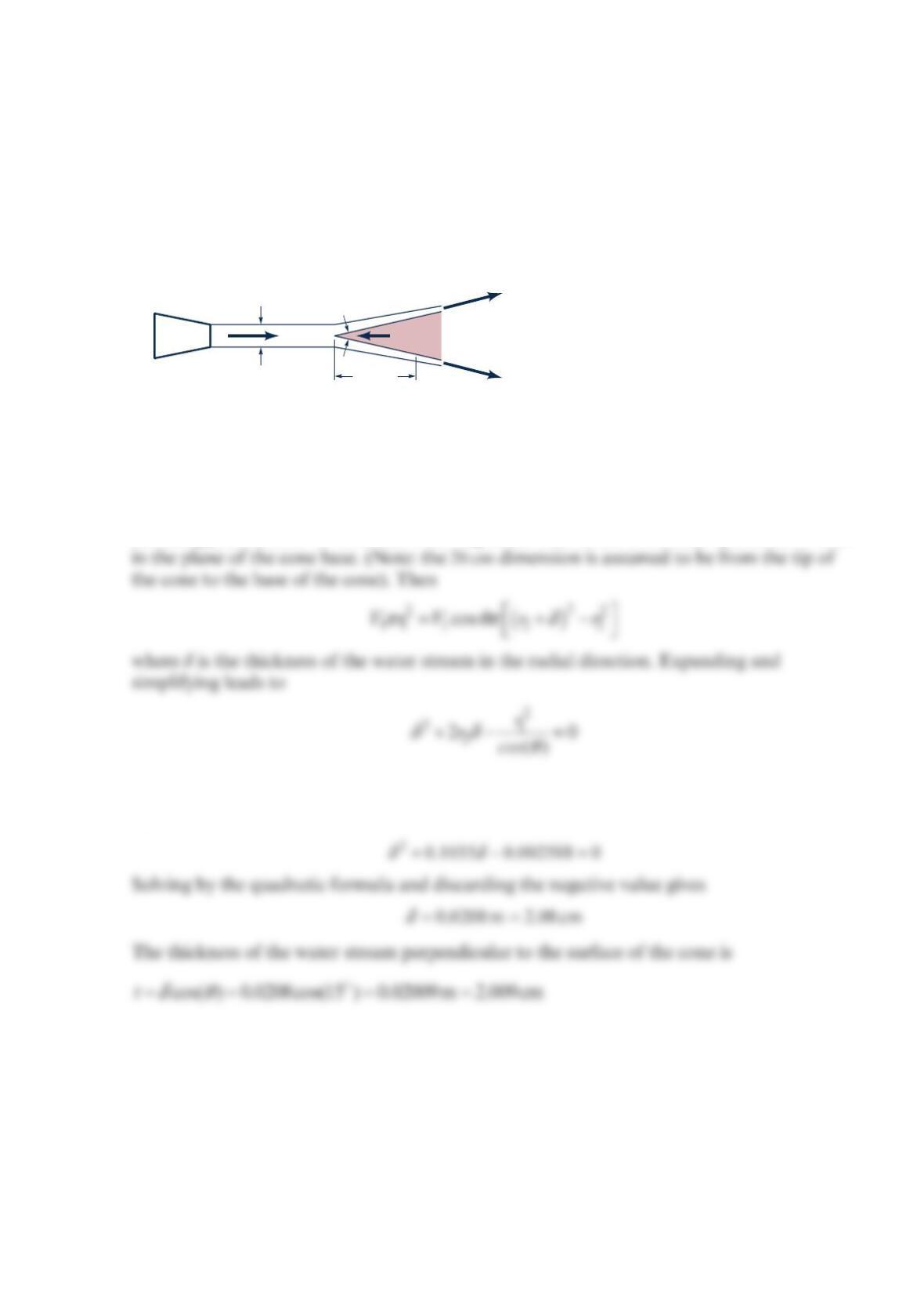
A water jet leaves a fixed nozzle with a velocity of 10 m/s. The jet diameter is 10 cm. A 30°
cone is pushed into the water jet at a speed of 5 m/s. The water impinges on the cone with
the jet axis and the cone axis in perfect alignment so that the water is divided evenly by the
cone. Bernoulli’s equation suggests that because the pressure on the jet boundary is
constant, the water velocity relative to the cone surface is constant. Determine the thickness
of the water stream when it reaches the base of the cone.
Solution 5.29
Consider a control volume attached to the cone. The water jet approaches this control
volume at 15 m/s. The continuity equation gives 11 2 2n
V
AVA= where location “1” is the
incoming jet, location “2” is the flow leaving at the base of the cone, and 2
A
is the flow area
For the situation in Fig. 5.29,
θ
== = =
12
0.05 m 0.20 sin(15 ) 0.05176 m 15rr
and the
equation becomes
20 cm
10 cm
10 m/s
30°
5 m/s
Problem 5.30
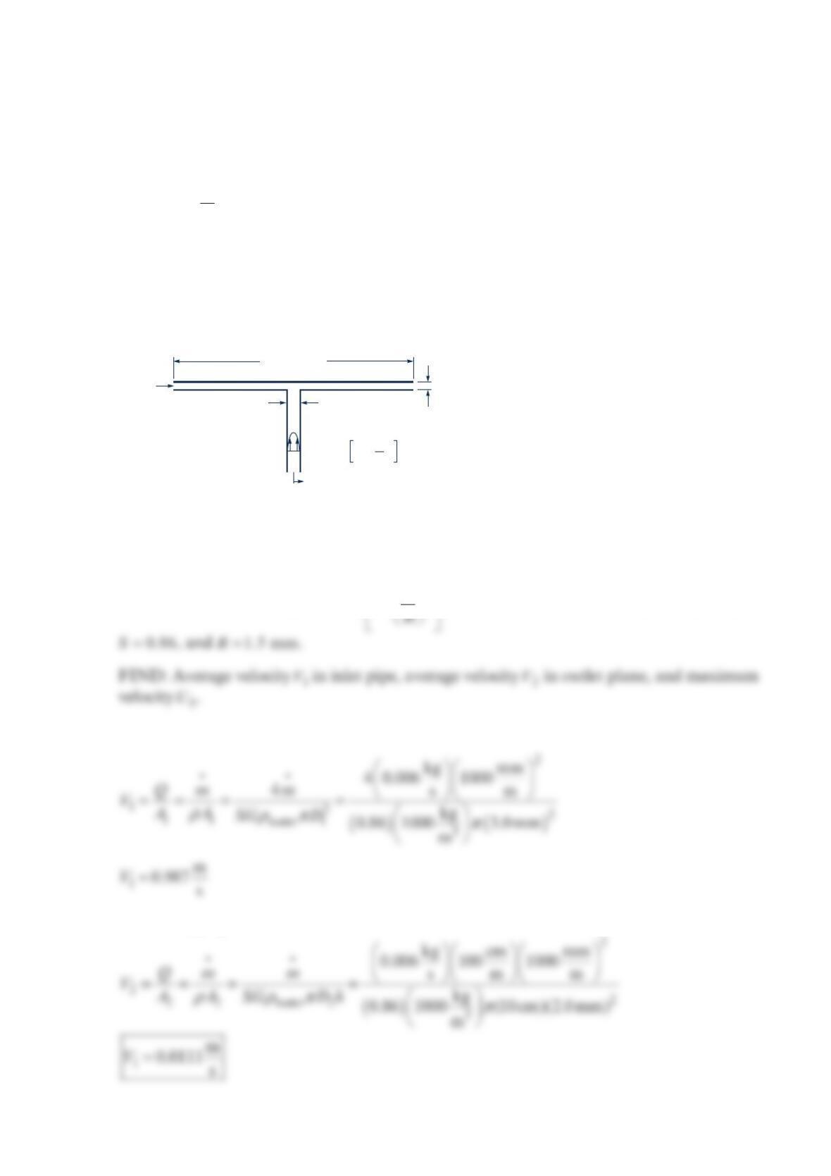
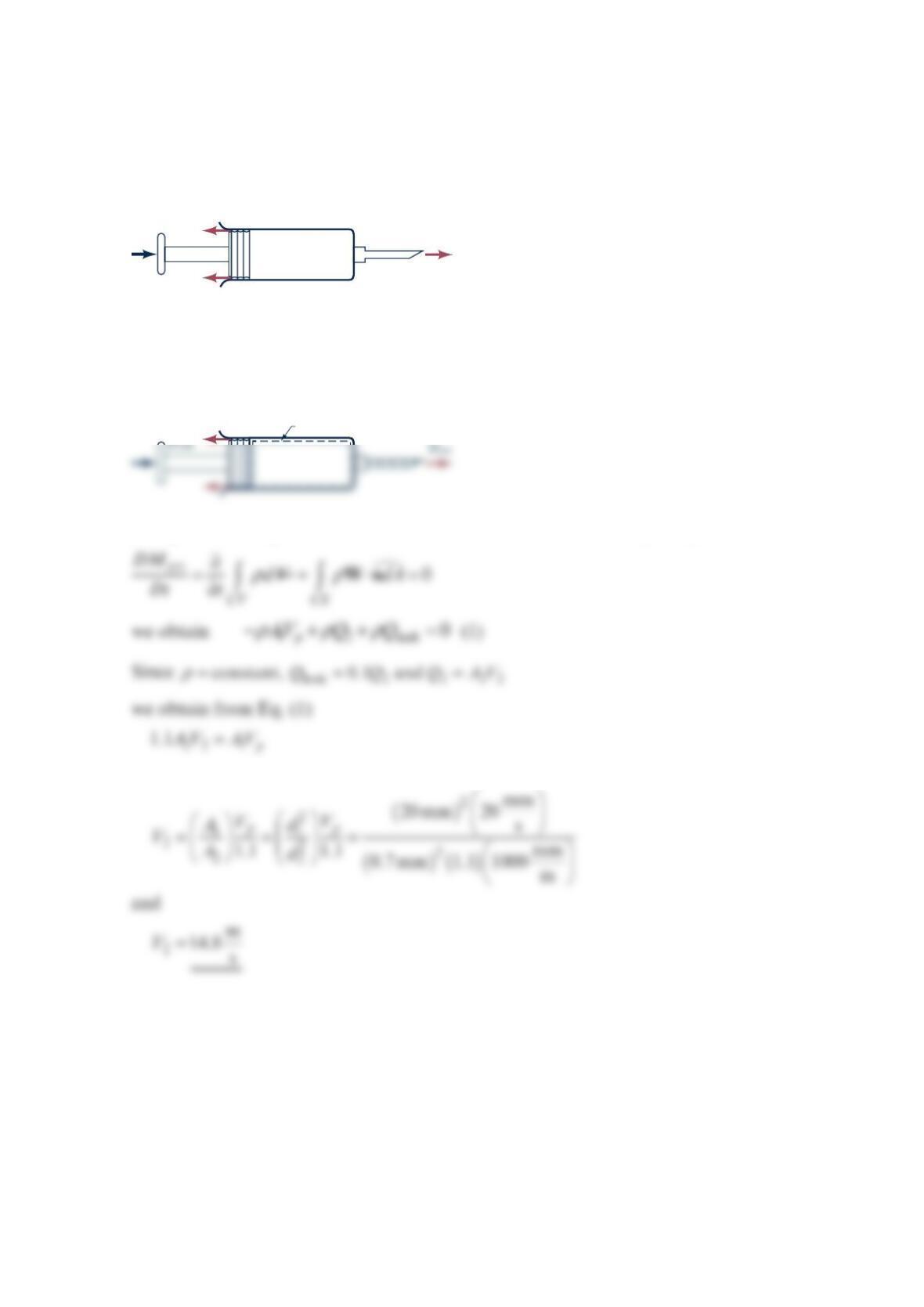
A hypodermic syringe (see the figure below) is used to apply a vaccine. If the plunger is
moved forward at the steady rate of 20 mm/s and if vaccine leaks past the plunger at 0.1 of
the volume flowrate out the needle opening, calculate the average velocity of the needle exit
flow. The inside diameters of the syringe and the needle are 20 mm and 0.7 mm.
Solution 5.30
Using a deforming control volume and the conservation of mass principle
or
Qleak Qout
Deforming control
volume
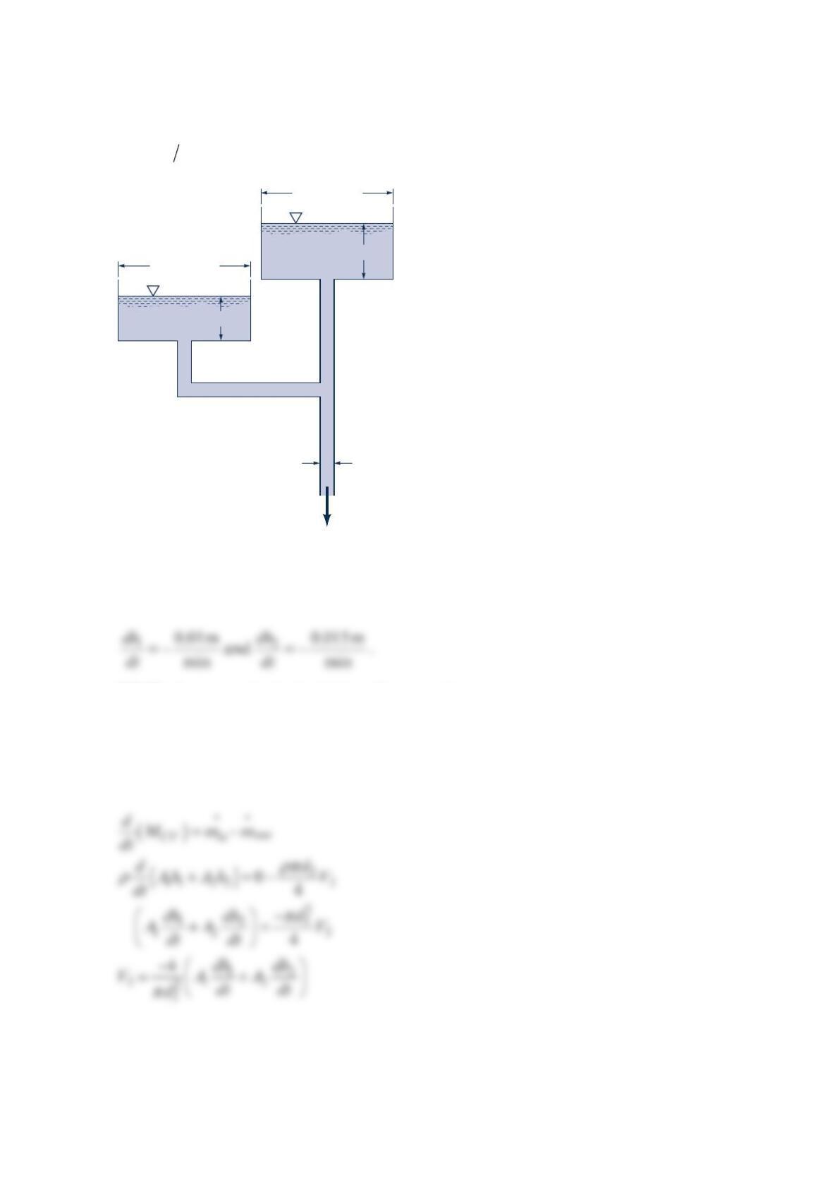
Problem 5.31
The figure below shows a two-reservoir water supply system. The water level in reservoir 1
drops at the rate of 0.01m/min , and the water level in reservoir 2 drops at the rate of
0.015 m min . Calculate the average velocity 3
V
in the 0.50-m-diameter pipe.
Solution 5.31
GIVEN: The figure with
FIND: Average velocity in 0.50 m diameter pipe.
SOLUTION:
Assume constant water density and apply conservation of mass to a control volume
enclosing the two tanks and the 0.50 m discharge pipe.
h1
A1
= 5 acres
Reservoir 1
h2
A2
= 4 acres
d3
= 0.50 m
V3
Reservoir 2
The numerical values give
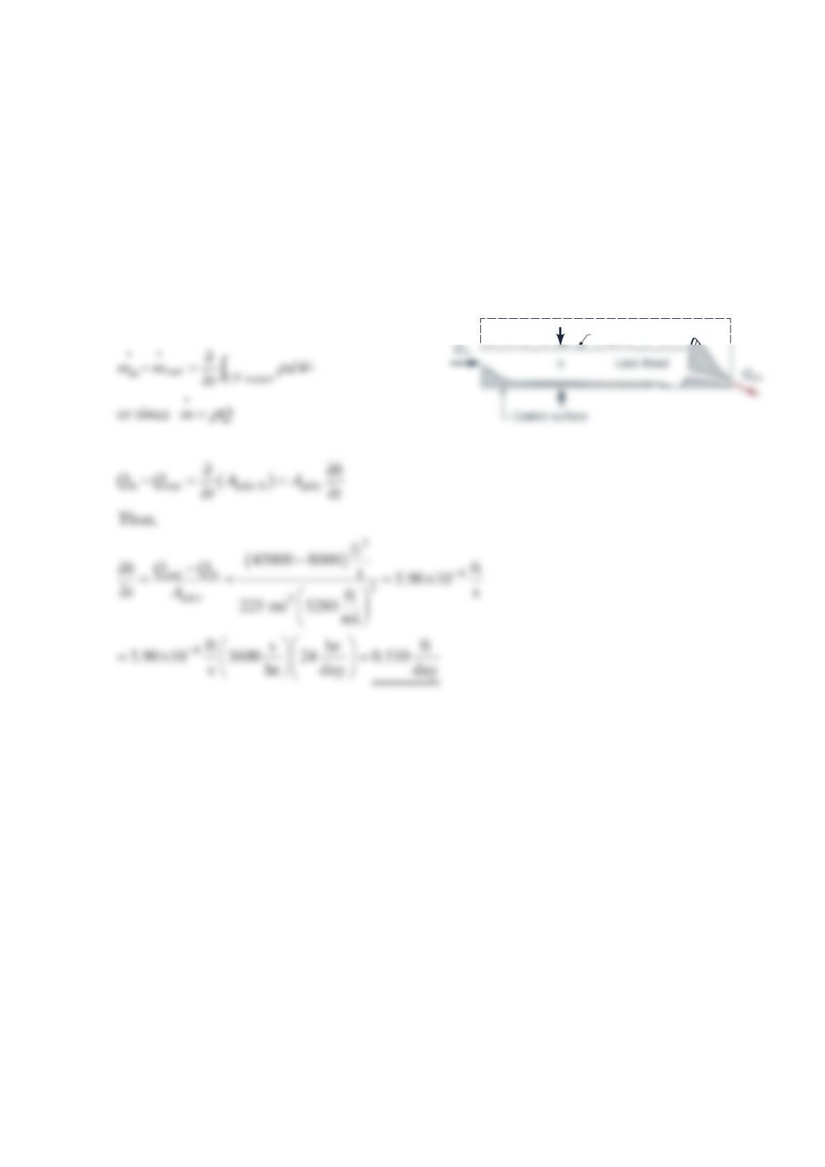
Problem 5.32
The Hoover Dam backs up the Colorado River and creates Lake Mead, which is
approximately
1
15 miles long and has a surface area of approximately
2
25 square miles. If
during flood conditions, the Colorado River flows into the lake at a rate of 45,000 cfs and
the outflow from the dam is
8
000 cfs, how many feet per 24-hour day will the lake level
rise?
Solution 5.32
For the control volume shown:
Alake
Problem 5.33
Storm sewer backup causes your basement to flood at the steady rate of
1
in. of depth per
hour. The basement floor area is 2
1500 ft . What capacity (gal mi
n
) pump would you rent
to (a) keep the water accumulated in your basement at a constant level until the storm
sewer is blocked off, and (b) reduce the water accumulation in your basement at a rate of
3
in. hr even while the backup problem exists?
Solution 5.33
For a deforming control volume that contains the water over the basement floor (see sketch
above), the conservation of mass principle sys
DM dV
Dt t
ρ
∂
=∂
CV CS
0dA
ρ
+⋅=
Wn leads to
(a) For part a, Eq. (1) leads to
Deforming
control volume that
contains water
h
(b) For part b, Eq. (1) yields
Problem 5.34
“Green” 1.6-gpf standards Toilets account for approximately 40% of all indoor household
water use. To conserve water, the new standard is 1.6 gallons of water per flush (gpf). Old
toilets use up to 7 gpf; those manufactured after 1980 use 3.5 gpf. Neither is considered a
low-flush toilet. A typical 3.2-person household in which each person flushes a 7-gpf toilet
4 times a day uses 32,700 gallons of water each year; with a 3.5-gpf toilet, the amount is
reduced to 16,400 gallons. Clearly the new 1.6-gpf toilets will save even more water.
However, designing a toilet that flushes properly with such a small amount of water is not
simple. Today there are two basic types involved: those that are gravity powered and those
that are pressure powered. Gravity toilets (typical of most currently in use) have rather long
cycle times. The water starts flowing under the action of gravity and the swirling vortex
motion initiates the siphon action that builds to a point of discharge. In the newer pressure-
assisted models, the flowrate is large, but the cycle time is short and the amount of water
used is relatively small. (See Problem 5.34.)
When a toilet is flushed, the water depth,
h
, in the tank as a function of time,
t
, is as given in
the table. The size of the rectangular tank is
1
9in.
by
7
.5 in. (a) Determine the volume of
water used per flush, gpf . (b) Plot the flowrate for ≤≤06st.
t (s) h (in.)
0 5.70
0.5 5.33
1.0 4.80
2.0 3.45
3.0 2.40
4.0 1.50
5.0 0.75
6.0 0
Solution 5.34
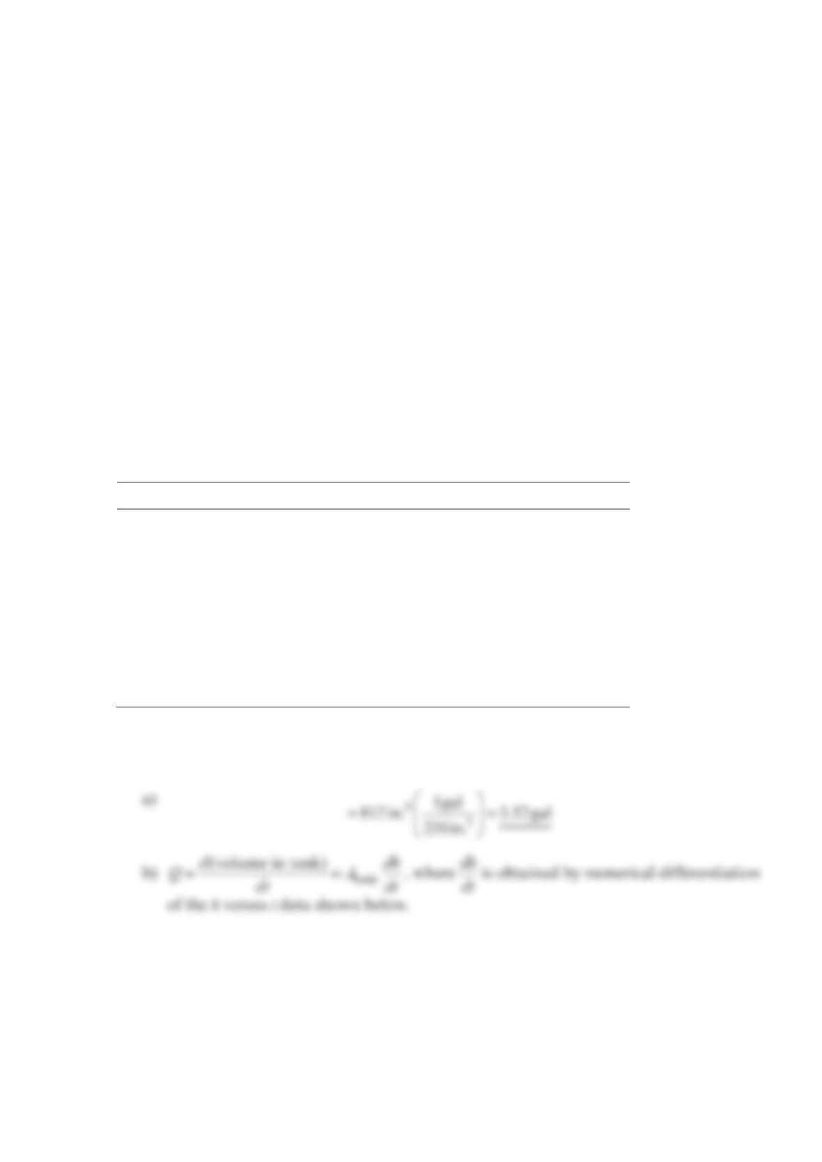
=×=
3
Volume of water per flush 5.70 in.(19 in. 7.5 in.) 812 in.
h
t
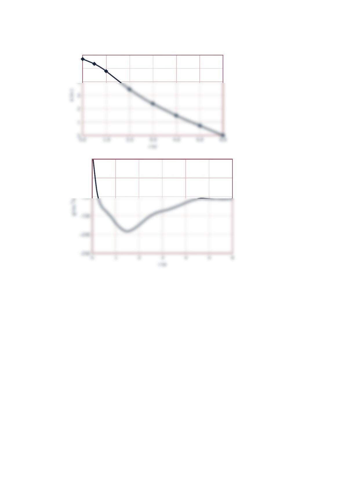
The resulting
Q
versus
t
result are also shown below.
6
5
0
–50