PROBLEM 5.91 (Cont.)
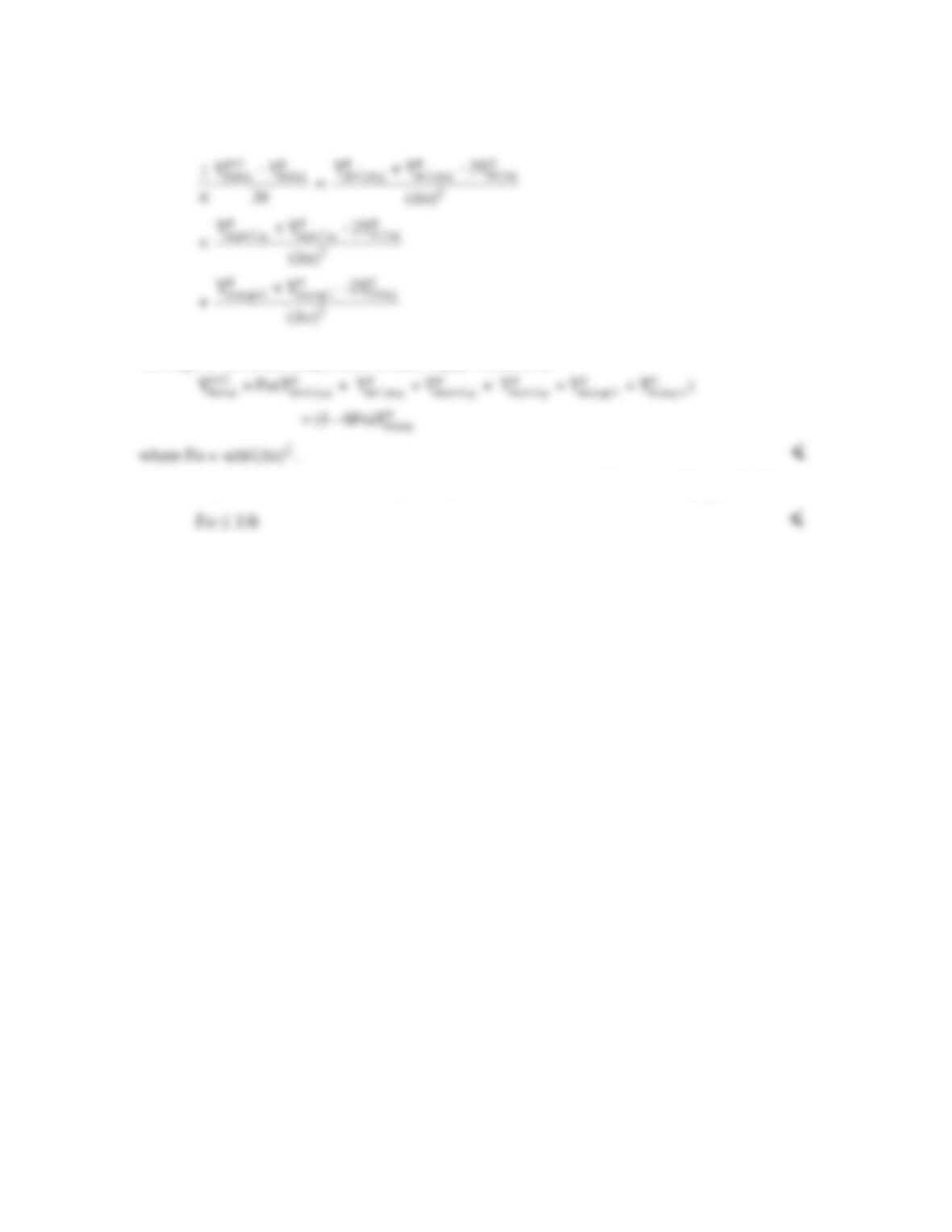
Solving for the nodal temperature at time step p+1 results in
The stability criterion is determined by the requirement that the coefficient of
p
m,n,q
T
≥ 0. Thus
COMMENTS: These results could also have been obtained using the energy balance method
applied to a control volume about the interior node.
PROBLEM 5.92
KNOWN: Nodal point located at boundary between two materials A and B.
FIND: Two-dimensional explicit, transient finite difference equation.
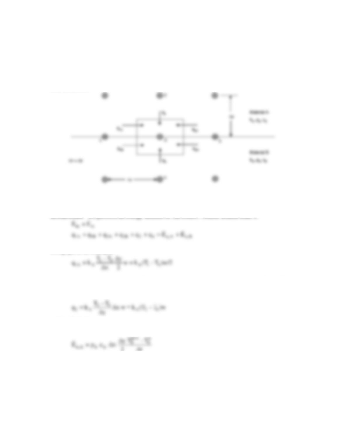
SCHEMATIC:
ASSUMPTIONS: (1) Two–dimensional conduction, (2) No heat generation, (3) Constant
properties (different in each material).
ANALYSIS: We perform an energy balance on the control volume around node 0.
Using q1A as an example,
where w is the depth into the page. The quantities q1B, q3A, and q3B can be found similarly. Then
q2 is given by
and similarly for q4.
The storage term
st,A
E
is given by
and similarly for
st,B
E
.
Combining equations yields
Continued….
PROBLEM 5.92 (Cont.)
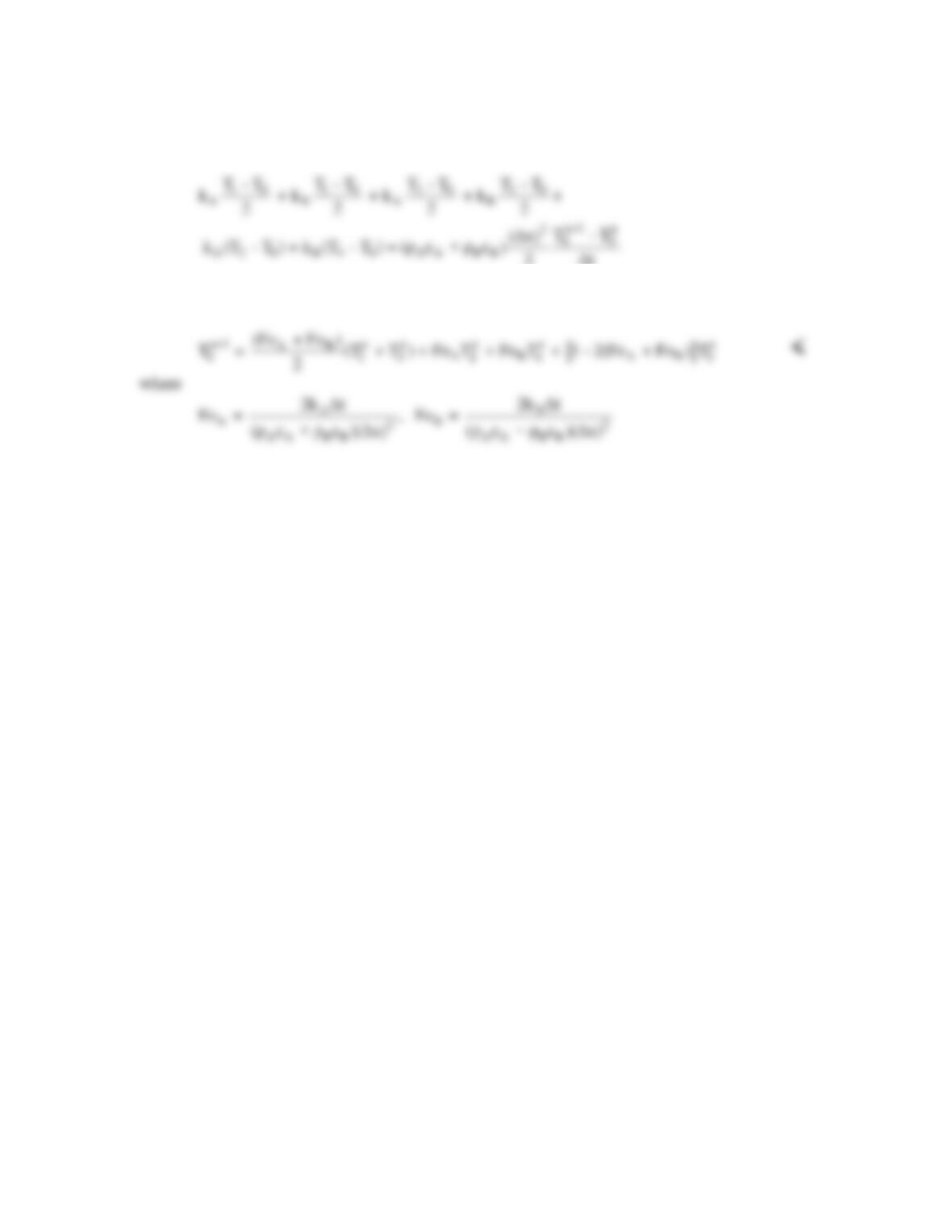
Rearranging, we find
Note, that
2
AA
Fo α Δt/(Δx)≠
.
COMMENTS: Note that when the material properties are the same for materials A and B, the
result agrees with Equation 5.79.
PROBLEM 5.93
KNOWN: A 0.12 m thick wall, with thermal diffusivity 1.5 × 10⁻⁶ m2/s, initially at a uniform
temperature of 85°C, has one face suddenly lowered to 20°C while the other face is perfectly insulated.
FIND: (a) Using the explicit finite–difference method with space and time increments of ∆x = 30 mm
and ∆t = 300s, determine the temperature distribution within the wall 45 min after the change in surface
temperature; (b) Effect of ∆t on temperature histories of the surfaces and midplane.
ASSUMPTIONS: (1) One-dimensional transient conduction, (2) Constant properties.
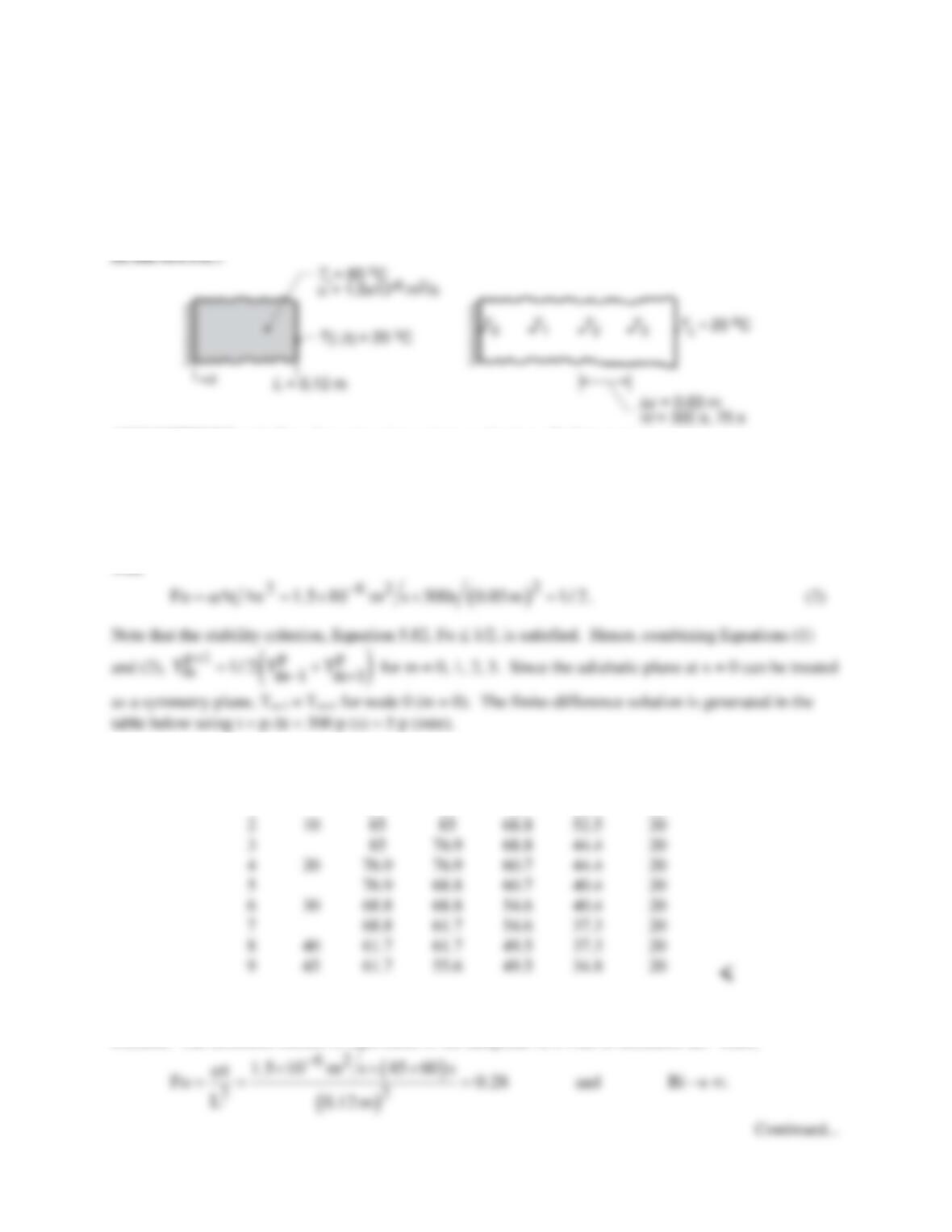
ANALYSIS: (a) The finite-difference equations for the interior points, nodes 0, 1, 2, and 3, can be
determined from Equation 5.81,
()
( )
p1 p p p
mm
m1 m1
T Fo T T 1 2 Fo T
+−+
= + +−
(1)
with
p
t(min)
T0
T1
T2
T3
TL(°C)
0
0
85
85
85
85
20
1
85
85
85
52.5
20
2
85
85
68.8
52.5
20
85
76.9
68.8
44.4
20
76.9
76.9
60.7
44.4
20
76.9
68.8
60.7
40.4
20
68.8
68.8
54.6
40.4
20
68.8
61.7
54.6
37.3
20
61.7
61.7
49.5
37.3
20
The temperature distribution can also be determined from the one-term approximation of the exact
solution. The insulated surface is equivalent to the midplane of a wall of thickness 2L. Thus,
PROBLEM 5.93 (Cont.)
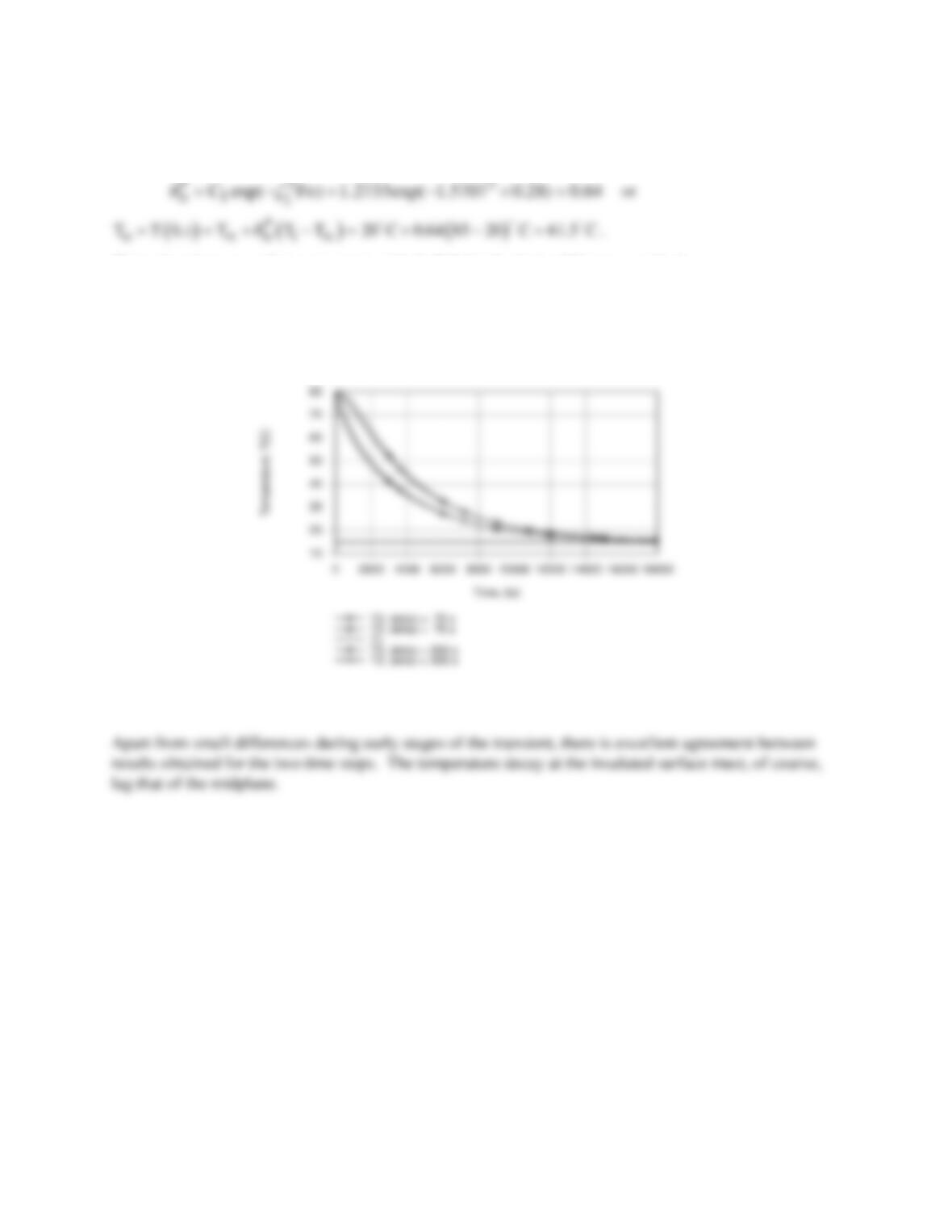
From Table 5.1, ζ1 = 1.5707, C1 = 1.2733. Then from Equation 5.44,
This value shows excellent agreement with 61.7°C for the finite-difference method.
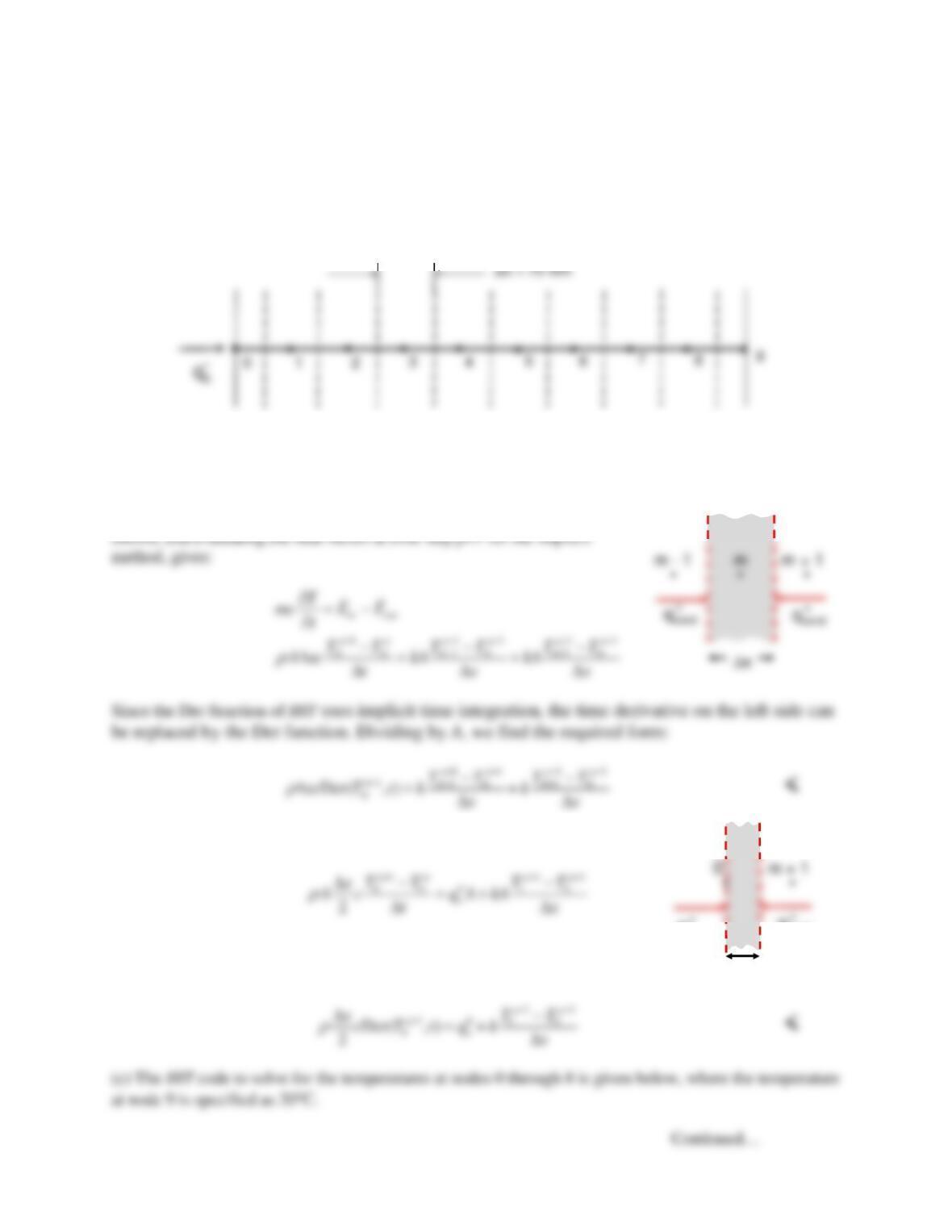
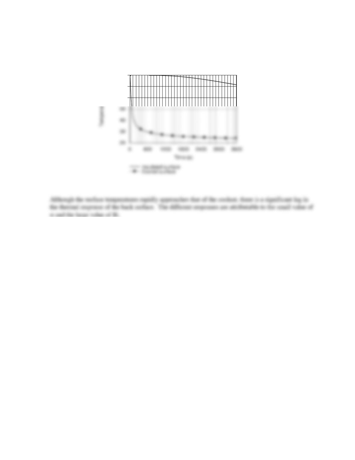
(b) Using the IHT Finite-Difference Equation Tool Pad for One–Dimensional Transient Conduction,
temperature histories were computed and results are shown for the insulated surface (T0) and the
midplane, as well as for the chilled surface (TL).
PROBLEM 5.94
KNOWN: Initial temperature of thick slab of copper. Surface heat flux.
FIND: (a) Expression for implicit finite-difference equations for interior nodes using the Der function of
IHT. (b) Expression for implicit finite-difference equations for surface node using the Der function of
IHT. (c) Nodal temperatures at t = 120 s.
SCHEMATIC:
ASSUMPTIONS: (1) Uniform properties, (2) One-dimensional conduction.
PROPERTIES: Table A-1, Copper, (T = 300 K): k = 401 W/m⋅K,
α
= 117 × 10−6 m2/s.
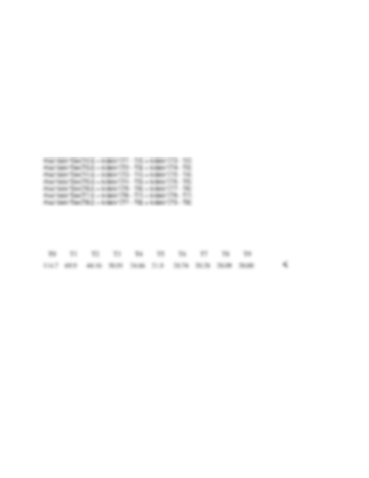
ANALYSIS: (a) Performing an energy balance on an interior node m, as
(b) For the surface node 0, an energy balance gives:
Replacing the derivative on the left with the Der function and dividing
by A gives:
q
o
″q
cond
″
∆x/2
PROBLEM 5.94 (Cont.)
//Example 5.12 using Der function of IHT
//Properties, dimensions, heat flux
k = 401
alpha = 117e-6
rhoc = k/alpha
qflux = 3e5
delx = 0.075
//Node 0
rhoc*delx/2*Der(T0,t) = qflux + k*(T1 – T0)/delx
//Nodes 1 through 8
rhoc*delx*Der(T1,t) = k/delx*(T0 – T1) + k/delx*(T2 – T1)
//Node 9
T9 = 20
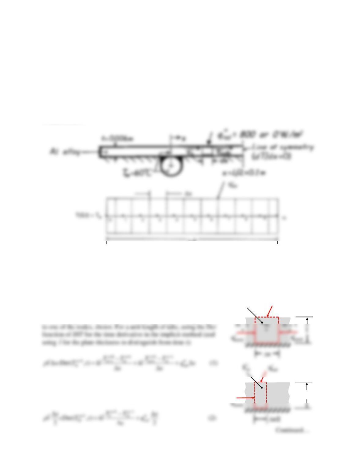
With initial temperatures of 20°C and a time step of 24 s, the solution at t = 120 s is:
COMMENTS: The solution using the Der function of IHT agrees almost exactly with the solution of the
implicit finite–difference equations in Example 5.12 for Fo = ½ (∆t = 24 s), as it should.
PROBLEM 5.95
KNOWN: Thickness of aluminum alloy (2024-T6) absorber plate. Spacing of tubes attached to plate,
temperature of plate at tube location. Net radiation heat flux.
FIND: (a) Steady–state temperature distribution and rate of thermal energy delivered to a tube per unit
length, using finite difference model, for
rad
q′′ =
800 W/m2. Maximum plate temperature. (b) Temperature
distribution for the 500 s time period after
rad
q′′
is reduced to zero. Plot of maximum plate temperature vs.
time. Values of maximum plate temperature for t = 0, 10, and 100 s. (c) Plot of heat transfer rate to tube
per unit length for the 500 s time period. Time for heat transfer rate to tube to be reduced by 50%.
SCHEMATIC:
L/2
ASSUMPTIONS: (1) Uniform properties, (2) Negligible temperature variation through plate thickness,
(3) Uniform radiation absorption at plate surface, (4) Negligible losses by conduction through insulation,
(5) Negligible losses by convection at absorber plate surface, (6) Temperature of absorber plate at x = 0 is
approximately that of the water.
PROPERTIES: Table A–1, Aluminum alloy (2024-T6), (T = 325 K):
ρ
= 2770 kg/m3, cp = 873 J/kg⋅K, k
= 177 W/m⋅K,
α
= 7.33 × 10⁻⁵ m2/s.
ANALYSIS: The absorber plate acts as an extended surface. Finite
difference equations may be obtained by applying an energy balance
For Node 10, shown, which is at the symmetry plane between tubes,
there is zero heat flux into the control volume through the symmetry
plane. Thus the finite difference equation is:
•9
t
~
10
•
E
st
∙
q
rad
′
′
PROBLEM 5.95 (Cont.)
The heat transfer rate to a tube can be determined from an energy balance about Node 0, where the factor
of 2 accounts for heat coming from both directions (right and left):
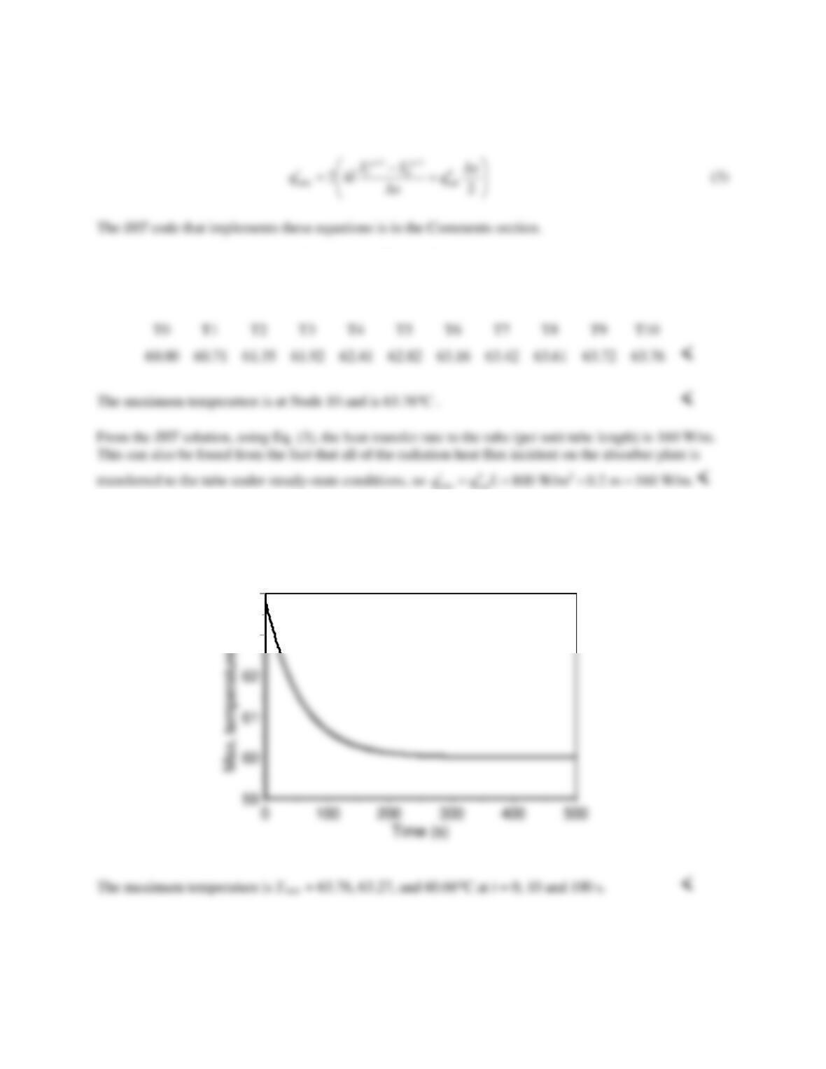
(a) For part (a), the radiation heat flux is set to 800 W/m2 and the solution is advanced until a steady–state
is reached. Alternatively, there is an analytical solution to the steady–state case, see Problem 3.89. The
steady–state solution from the IHT code is:
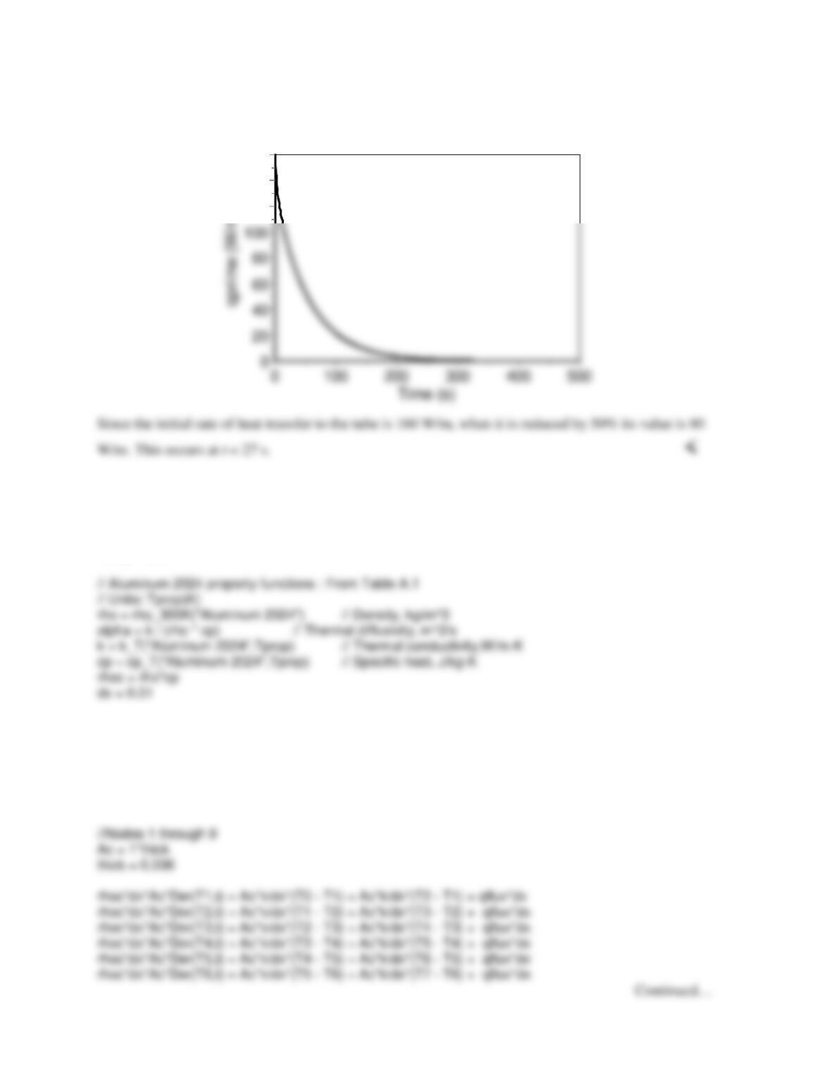
(b) Starting from the steady-state temperature distribution, the IHT code is run with zero radiation heat
flux and a time step of 1 s. A plot of the maximum temperature (at Node 10) as a function of time is given
below.
64
63
Continued…
PROBLEM 5.95 (Cont.)
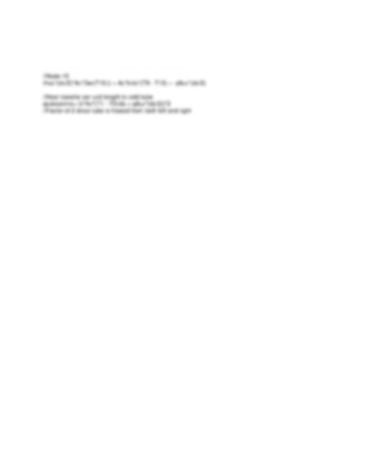
(c) The plot of the heat transfer rate to the tube per unit length, as a function of time, is shown below.
160
140
120
COMMENTS: (1) The IHT code that implements Eqs. (1-3) is given below.
//Properties,dimensions
//Properties at 325 K
Tprop = 325
//Radiative conditions
//qflux = 800 //Use for part (a) and run to steady–state.
qflux = 0 //Use for parts (b) and (c).
//Node 0
T0 = 60
PROBLEM 5.95 (Cont.)
rhoc*dx*Ac*Der(T7,t) = Ac*k/dx*(T6 – T7) + Ac*k/dx*(T8 – T7) + qflux*dx
rhoc*dx*Ac*Der(T8,t) = Ac*k/dx*(T7 – T8) + Ac*k/dx*(T9 – T8) + qflux*dx
rhoc*dx*Ac*Der(T9,t) = Ac*k/dx*(T8 – T9) + Ac*k/dx*(T10 – T9) + qflux*dx
PROBLEM 5.96
KNOWN: Thickness, initial temperature and thermophysical properties of molded plastic part.
Convection conditions at one surface. Other surface insulated.
FIND: Surface temperatures after one hour of cooling.
SCHEMATIC:
ASSUMPTIONS: (1) One-dimensional conduction in product, (2) Negligible radiation, at cooled
surface, (3) Negligible heat transfer at insulated surface, (4) Constant properties.
ANALYSIS: Adopting the implicit scheme, the finite-difference equation for the cooled surface
node is given by Eq. (5.96), from which it follows that
The general form of the finite-difference equation for any interior node (1 to 9) is given by Eq. (5.97),
For the prescribed conditions, Bi = h∆x/k = 100 W/m2⋅K (0.006m)/0.30 W/m⋅K = 2. If the explicit
method were used, the most restrictive stability requirement would be given by Eq. (5.87). Hence, for
Fo (1+Bi) ≤ 0.5, Fo ≤ 0.167. With Fo = α∆t/∆x2 and α = k/ρc = 1.67 ×10⁻⁷ m2/s, the corresponding
COMMENTS: (1) More accurate results may be obtained from the one–term approximation to the
exact solution for one-dimensional, transient conduction in a plane wall. With Bi = hL/k = 20, Table
5.1 yields
1
ζ
= 1.496 rad and C1 = 1.2699. With Fo = αt/L2 = 0.167, Eq. (5.41) then yields To = T∞
PROBLEM 5.96 (Cont.)
(2) Temperature histories for the front and back surface nodes are as shown.
60
70
80
PROBLEM 5.97
KNOWN: Thickness and thermal diffusivity of a plane wall. Initial and boundary conditions.
FIND: (a) Time required for the left face temperature to reach 50% of its maximum possible
temperature reduction and (b) Time required for the left face temperature to recover to a 20%
temperature reduction when the right face temperature is returned to its initial value.
SCHEMATIC:
ASSUMPTIONS: (1) One-dimensional heat transfer, (2) Constant properties.
PROPERTIES: Thermal diffusivity,
= 6 10-7 m2/s (given).
ANALYSIS: Using the IHT Finite-Difference Equation Tool Pad for One-Dimensional Transient
Conduction, the following temperatures may be computed using the IHT code in the Comments
section. Note that for this solution, the conditions at the right face have been incorporated by
specifying a very large convection coefficient at the right face so that T5 T.
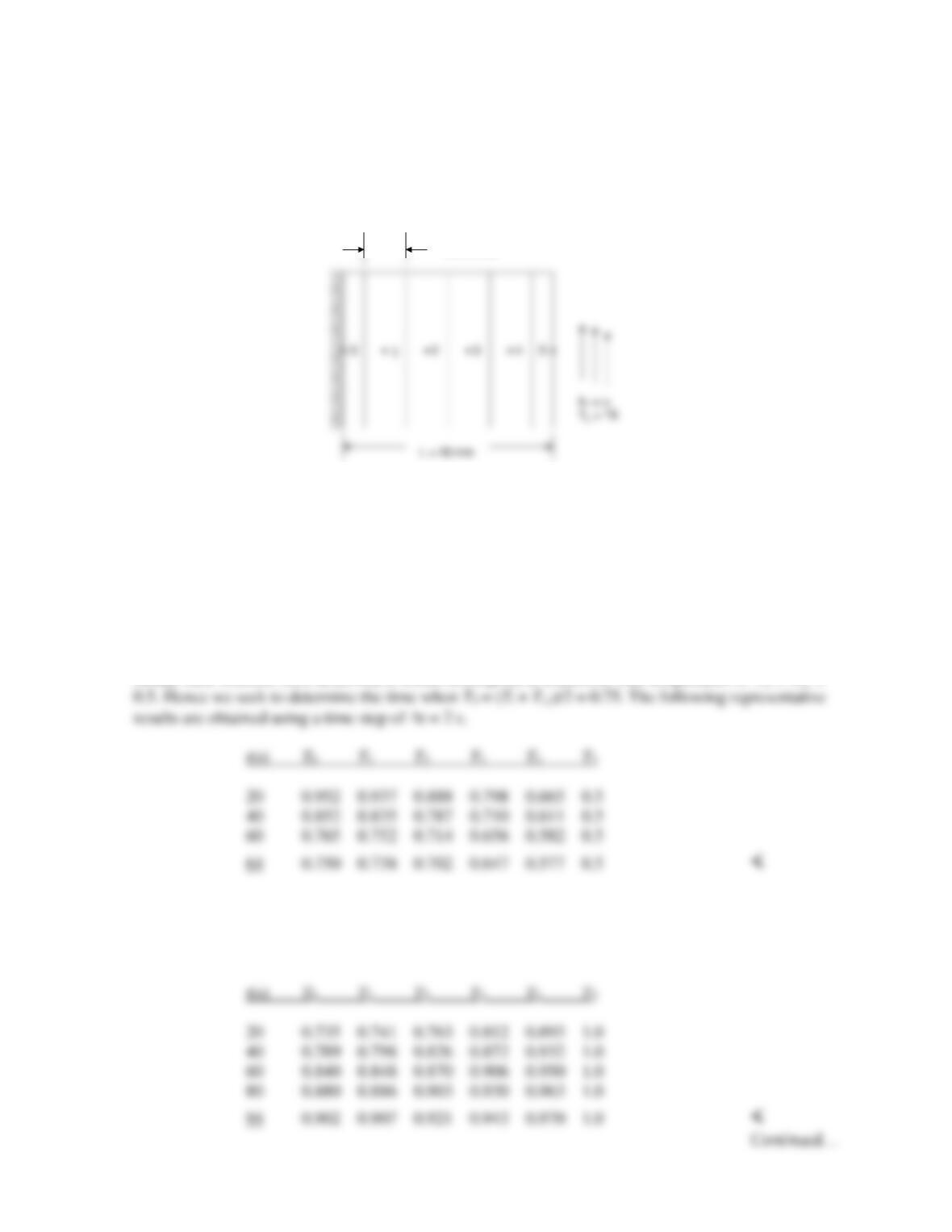
(a) For cooling conditions, the initial temperature is arbitrarily set to unity, and T = Ts,r = 0.5. If a
steady-state solution were achieved, it would correspond to a uniform wall temperature of Tss = Ts,r =
(b) For the heating conditions, we set the initial conditions in IHT to the temperatures shown at t = 64
in the table above. We set T = 1 and monitor the transient response of the system. The following
representative results are obtained.
x = 2 mm
x = 2 mm
PROBLEM 5.97 (Cont.)
COMMENTS: (1) The IHT Code for cooling and heating is shown below. (2) Note the thermal
response of T0 after heating ensues at the right face. The value of T0 continues to decrease for a short
time before it begins to increase in value. Does this make sense to you? (3) Part (a) can be solved
analytically using the one-term approximation, yielding t = 63 s. The numerical and analytical
solutions are in agreement to within an uncertainty associated with the time step of t = 2 s.
/* Node 0: surface node (w-orientation); transient conditions; e labeled 1. */
rho * cp * der(T0,t) = fd_1d_sur_w(T0,T1,k,qdot,deltax,Tinf,h1,qfla0)
/* Node 5: surface node (e-orientation); transient conditions; w labeled 4. */
rho * cp * der(T5,t) = fd_1d_sur_e(T5,T4,k,qdot,deltax,Tinf,h2,qfla5)
// Cooling
//Tinf = 0.5 //Initial Conditions are T = 1.0 everywhere.
//Heating //Initial Conditions are the temperatures at t = 64 s.
Tinf = 1.0
PROBLEM 5.98
KNOWN: Fuel element of Example 5.11 is initially at a uniform temperature of 250°C with
no internal generation; suddenly a uniform generation,
83
q 10 W/m ,=
occurs when the
element is inserted into the core while the surfaces experience convection (T∞,h).
FIND: Temperature distribution 1.5s after element is inserted into the core.
SCHEMATIC:
ASSUMPTIONS: (1) One-dimensional transient conduction, (2) Constant properties, (3)
q 0,=
initially; at t > 0,
q
is uniform.
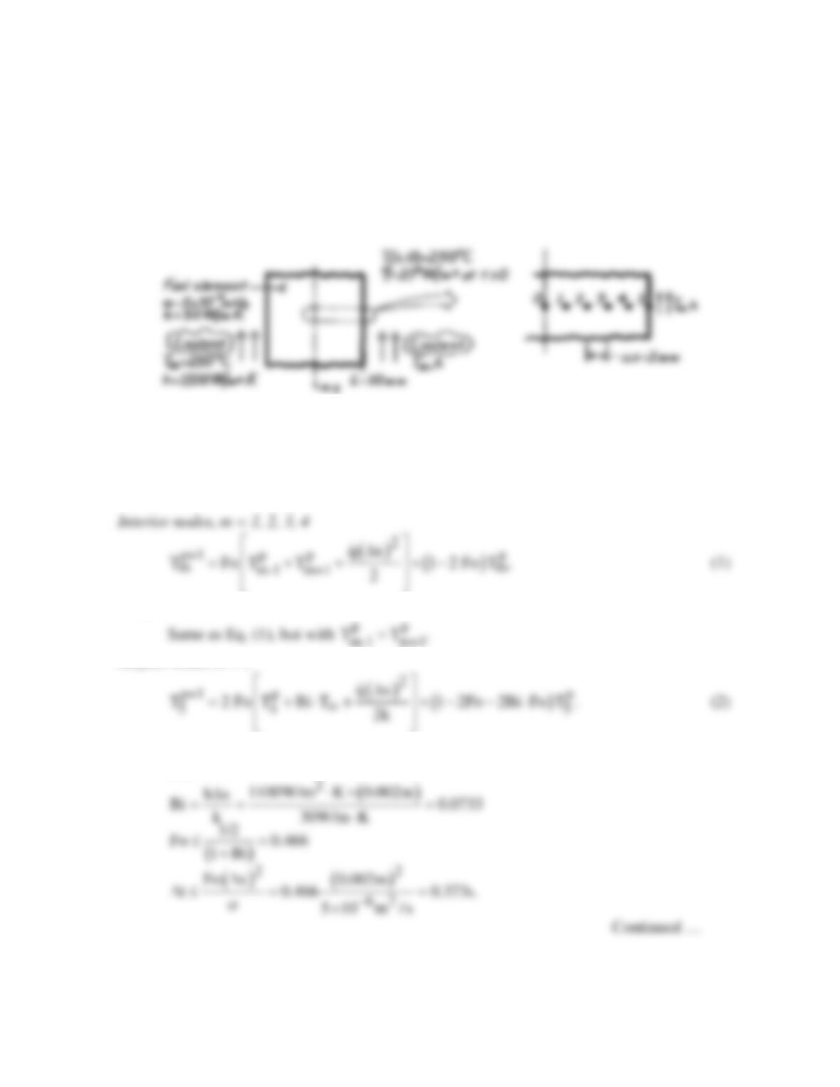
ANALYSIS: As suggested, the explicit method with a space increment of 2mm will be used.
Using the nodal network of Example 5.11, the same finite–difference equations may be used.
Midplane node, m = 0
Surface node, m = 5
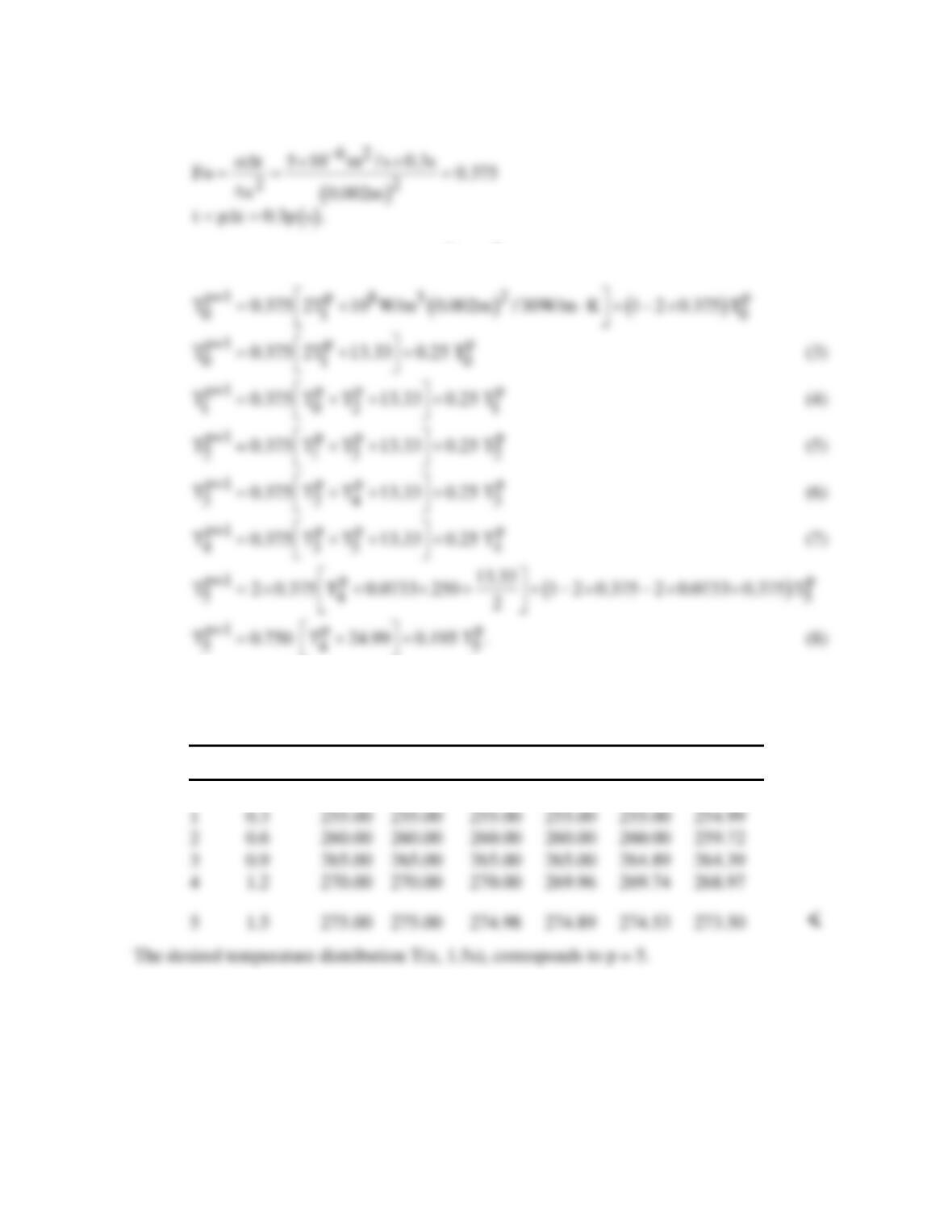
The most restrictive stability criterion is associated with Eq. (2), Fo(1+Bi) ≤ 1/2. Consider the
following parameters:
PROBLEM 5.98 (Cont.)
To be well within the stability limit, select ∆t = 0.3s, which corresponds to
Substituting numerical values with
83
q 10 W/m ,=
the nodal equations become
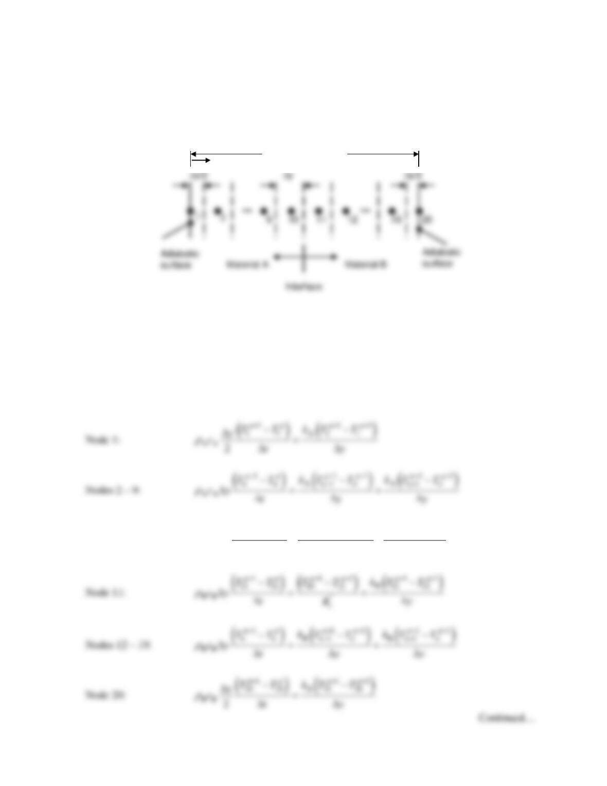
The initial temperature distribution is Ti = 250°C at all nodes. The marching solution,
following the procedure of Example 5.11, is represented in the table below.
p t(s) T0 T1 T2 T3 T4 T5(°C)
0 0 250 250 250 250 250 250
COMMENTS: Note that the nodes near the midplane (0,1) do not feel any effect of the
coolant during the first 1.5s time period.
PROBLEM 5.99
KNOWN: Dimensions and properties of acrylic and steel plates. Initial temperatures.
FIND: Time needed to bring external surface of the acrylic to its softening temperature. Plot of the
average acrylic and steel plate temperatures and acrylic surface temperature for 0 ≤ t ≤ 300 s.
SCHEMATIC:
ASSUMPTIONS: (1) One–dimensional conduction, (2) Constant properties, (3) Negligible contact
resistance.
PROPERTIES: Acrylic (given):
ρ
A = 1990 kg/m3, cA = 1470 J/kg⋅K and kA = 0.21 W/m⋅K. Steel
(given):
ρ
B = 7800 kg/m3, cB = 500 J/kg⋅K and kB = 45 W/m⋅K.
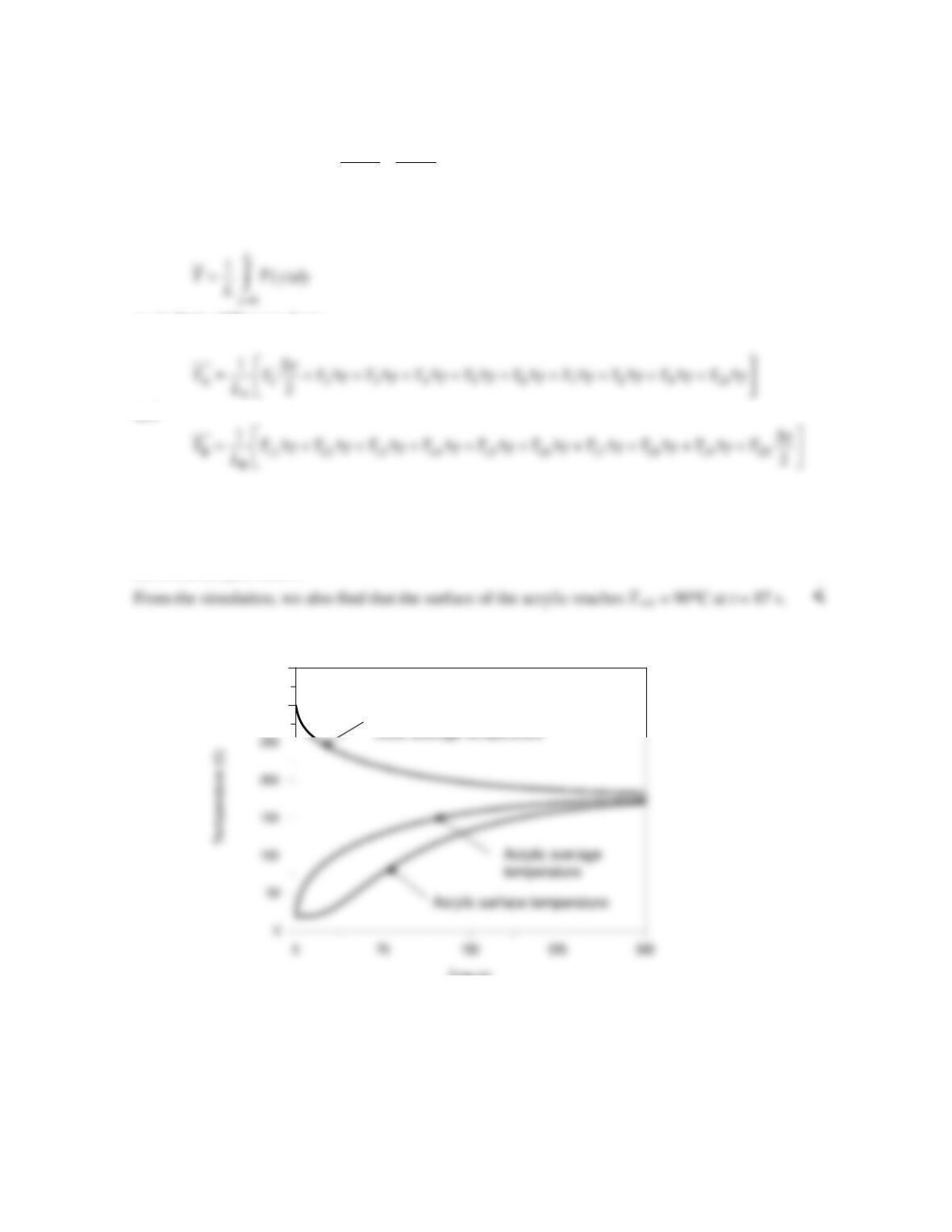
ANALYSIS: We begin by writing energy balances on each of the 20 control volumes using the
implicit method,
Node 10:
( ) ( ) ( )
1 11 11
A
10 10 9 10 11 10
AA “
pp pp pp
t
TTkTT TT
cy ty
R
ρ
+ ++ ++
− −−
∆= +
∆∆
y2L = 10 mm
PROBLEM 5.99 (Cont.)
where
“
AB
/2 /2
t
yy
Rkk
∆∆
= +
Also, note that the average temperature of each material may be written as
or, in finite difference form,
and
The preceding equations were solved using IHT code that is listed in the Comments. The spatially-
averaged temperatures of the two plates, as well as the external temperature of the acrylic, T1, are
shown in the plot below. <
COMMENTS: (1) Ultimately, the temperatures of the two plates will reach the same steady–state
value. The steady-state temperature may be found by recognizing the energy gained by the acrylic is
lost by the steel, LAcA(Tss – Ti,A) = LBcB(Ti,B – Tss) yielding Tss = 180°C, as evident in the plot of the
average temperatures. (2) If the surface of the acrylic in contact with the metal is assumed to be of
constant temperature and equal to 300°C, the external surface of the acrylic reaches the softening
temperature at t = 74 s. (3) The IHT code is shown on the next page.
Continued…
Aver ag e Material and Acrylic Surface Temperatures
Time ( s)
300
350
PROBLEM 5.99 (Cont.)
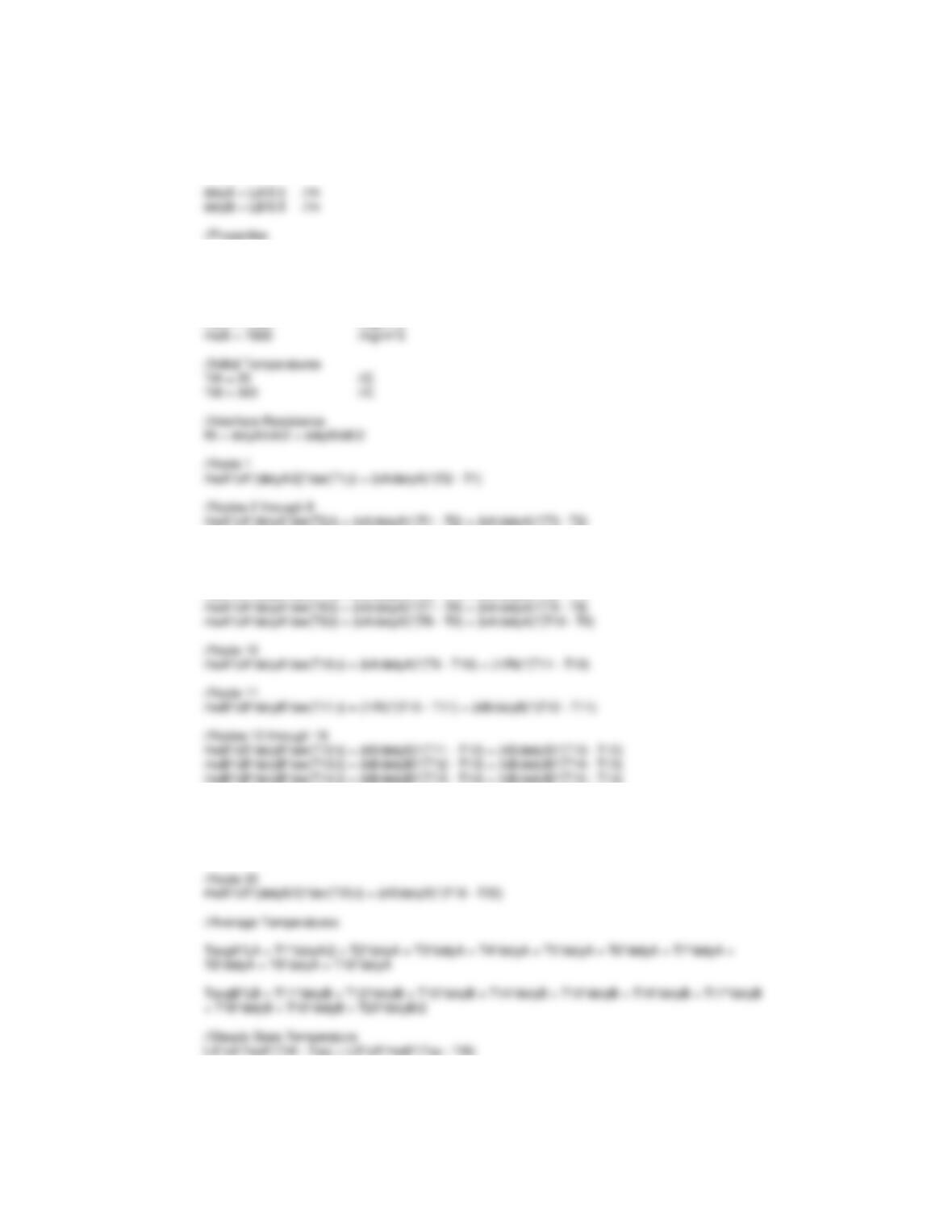
//Geometry and Discretization
LA = 0.005 //m
LB = 0.005 //m
kA = 0.21 //W/mK
kB = 45 //W/mK
cA = 1470 //J/kgK
cB = 500 //J/kgK
rhoA = 1990 //kg/m^3
rhoA*cA*delyA*der(T3,t) = (kA/delyA)*(T2 – T3) + (kA/delyA)*(T4 – T3)
rhoA*cA*delyA*der(T4,t) = (kA/delyA)*(T3 – T4) + (kA/delyA)*(T5 – T4)
rhoA*cA*delyA*der(T5,t) = (kA/delyA)*(T4 – T5) + (kA/delyA)*(T6 – T5)
rhoA*cA*delyA*der(T6,t) = (kA/delyA)*(T5 – T6) + (kA/delyA)*(T7 – T6)
rhoA*cA*delyA*der(T7,t) = (kA/delyA)*(T6 – T7) + (kA/delyA)*(T8 – T7)
rhoB*cB*delyB*der(T15,t) = (kB/delyB)*(T14 – T15) + (kB/delyB)*(T16 – T15)
rhoB*cB*delyB*der(T16,t) = (kB/delyB)*(T15 – T16) + (kB/delyB)*(T17 – T16)
rhoB*cB*delyB*der(T17,t) = (kB/delyB)*(T16 – T17) + (kB/delyB)*(T18 – T17)
rhoB*cB*delyB*der(T18,t) = (kB/delyB)*(T17 – T18) + (kB/delyB)*(T19 – T18)
rhoB*cB*delyB*der(T19,t) = (kB/delyB)*(T18 – T19) + (kB/delyB)*(T20 – T19)