PROBLEM 5.1
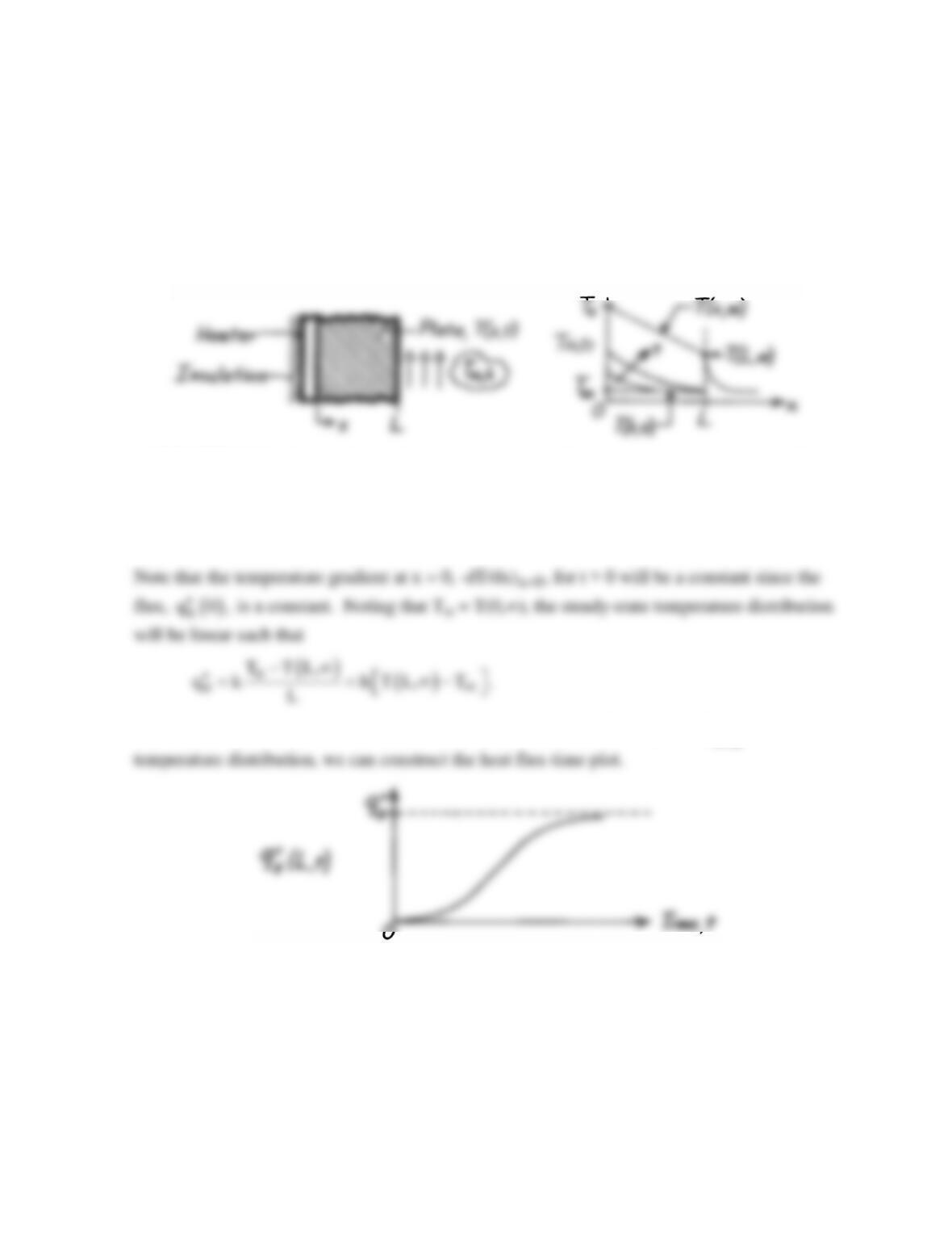
KNOWN: Electrical heater attached to backside of plate while front surface is exposed to
convection process (T∞,h); initially plate is at a uniform temperature of the ambient air and
suddenly heater power is switched on providing a constant
o
q.
′′
FIND: (a) Sketch temperature distribution, T(x,t), (b) Sketch the heat flux at the outer
surface,
( )
x
q L,t
′′
as a function of time.
SCHEMATIC:
ASSUMPTIONS: (1) One-dimensional conduction, (2) Constant properties, (3) Negligible
heat loss from heater through insulation.
ANALYSIS: (a) The temperature distributions for four time conditions including the initial
distribution, T(x,0), and the steady–state distribution, T(x,∞), are as shown above.
(b) The heat flux at the front surface, x = L, is given by
( ) ( )
xx=L
q L,t k dT/dx .
′′ = −
From the
COMMENTS: At early times, the temperature and heat flux at x = L will not change from
their initial values. Hence, we show a zero slope for
( )
x
q L,t
′′
at early times. Eventually, the
value of
( )
x
q L,t
′′
will reach the steady–state value which is
o
q.
′′
PROBLEM 5.2
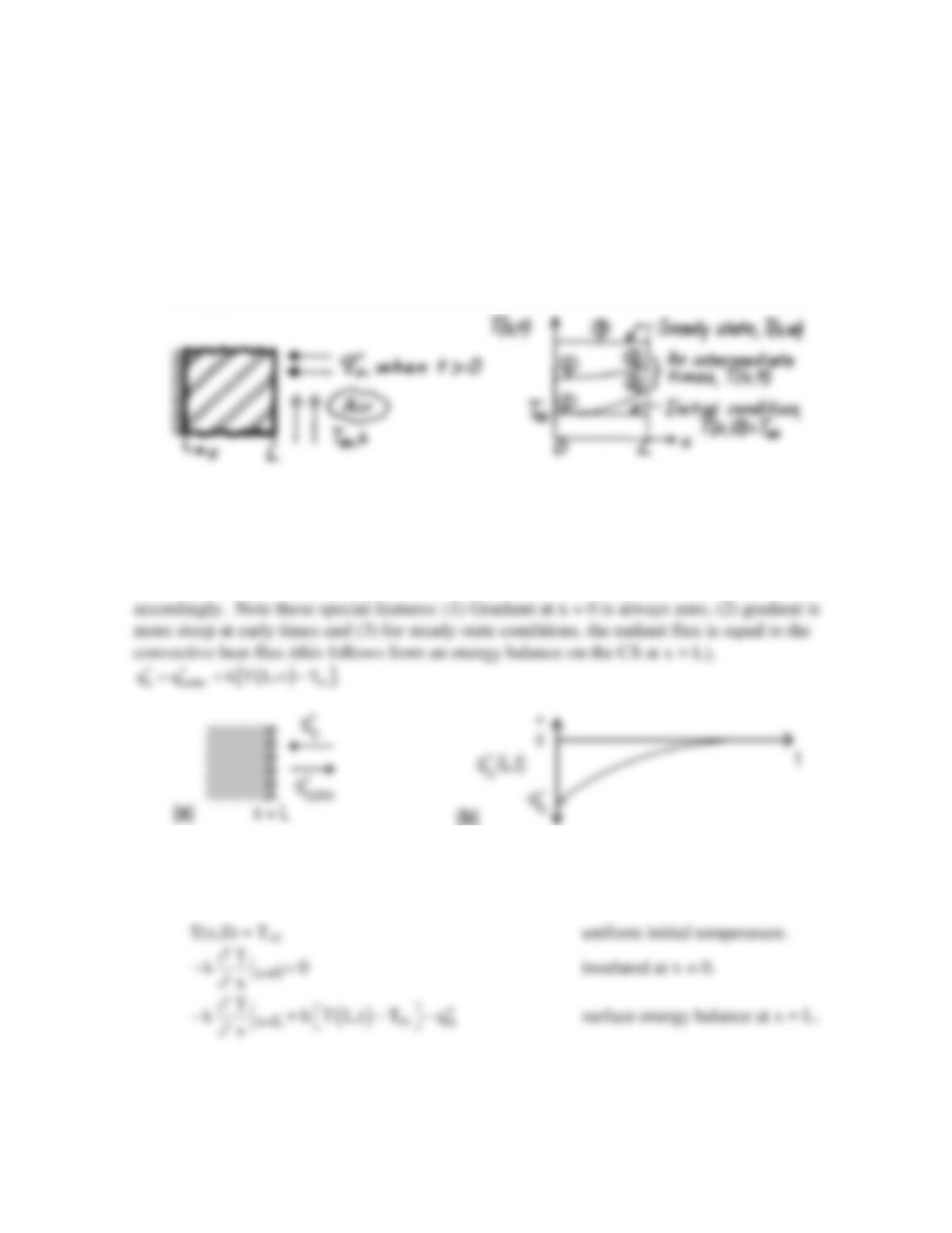
KNOWN: Plane wall whose inner surface is insulated and outer surface is exposed to an
airstream at T∞. Initially, the wall is at a uniform temperature equal to that of the airstream.
Suddenly, a radiant source is switched on applying a uniform flux,
o
q,
′′
to the outer surface.
FIND: (a) Sketch temperature distribution on T-x coordinates for initial, steady–state, and
two intermediate times, (b) Sketch heat flux at the outer surface,
( )
x
q L,t ,
′′
as a function of
time.
SCHEMATIC:
ASSUMPTIONS: (1) One-dimensional conduction, (2) Constant properties, (3) No internal
generation,
g
E 0,=
∀
(4) Surface at x = 0 is perfectly insulated, (5) All incident radiant power
is absorbed and negligible radiation exchange with surroundings.
ANALYSIS: (a) The temperature distributions are shown on the T-x coordinates and labeled
(b) The heat flux at the outer surface,
( )
x
q L,t ,
′′
as a function of time appears as shown above.
COMMENTS: The sketches must reflect the initial and boundary conditions:
PROBLEM 5.3
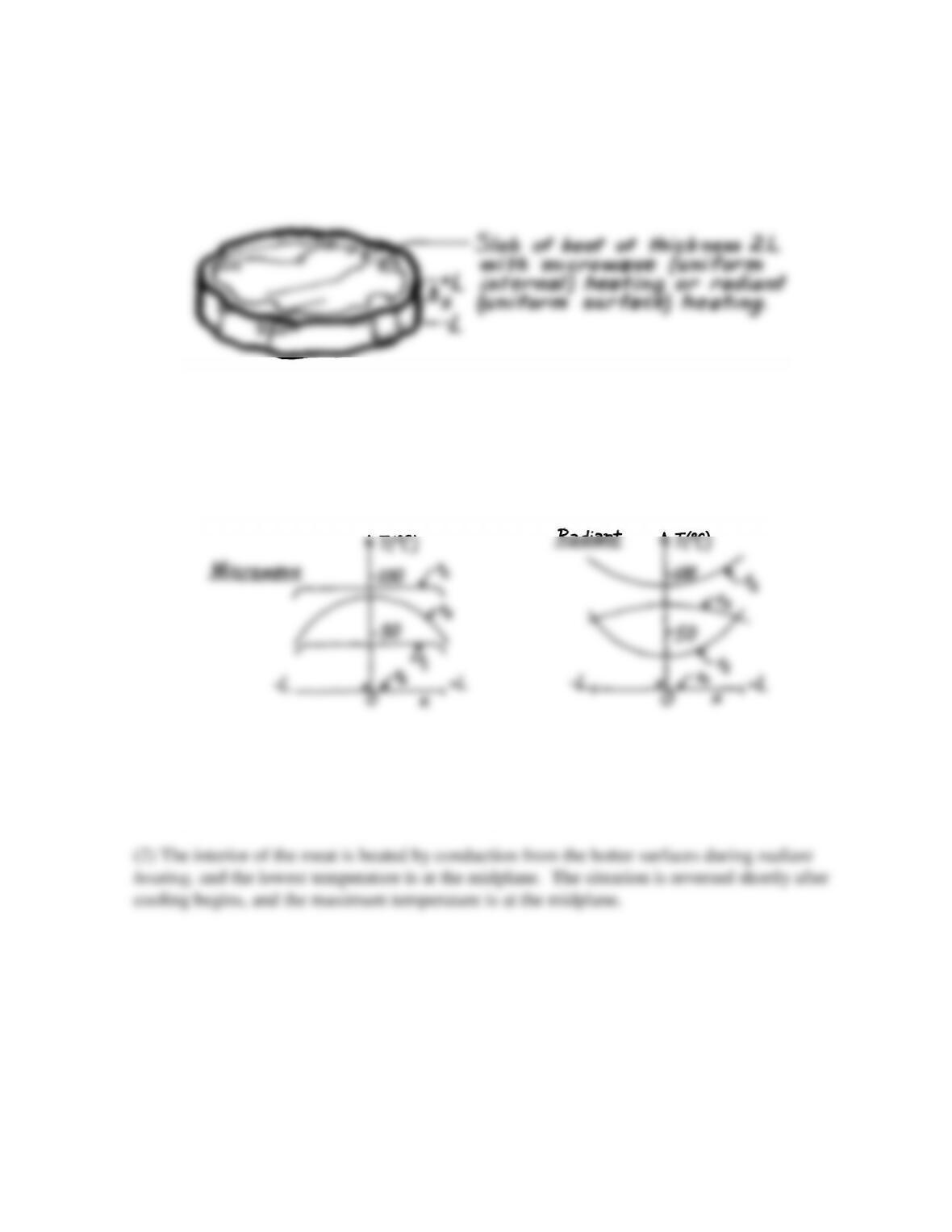
KNOWN: Microwave and radiant heating conditions for a slab of beef.
FIND: Sketch temperature distributions at specific times during heating and cooling.
SCHEMATIC:
ASSUMPTIONS: (1) One-dimensional conduction in x, (2) Uniform internal heat
generation for microwave, (3) Uniform surface heating for radiant oven, (4) Heat loss from
surface of meat to surroundings is negligible during the heating process, (5) Symmetry about
midplane.
ANALYSIS:
COMMENTS: (1) With uniform generation and negligible surface heat loss, the temperature
distribution remains nearly uniform during microwave heating. During the subsequent surface
cooling, the maximum temperature is at the midplane.
PROBLEM 5.4
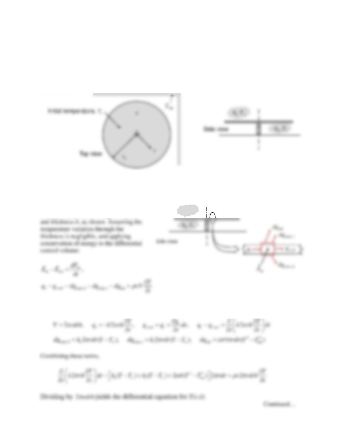
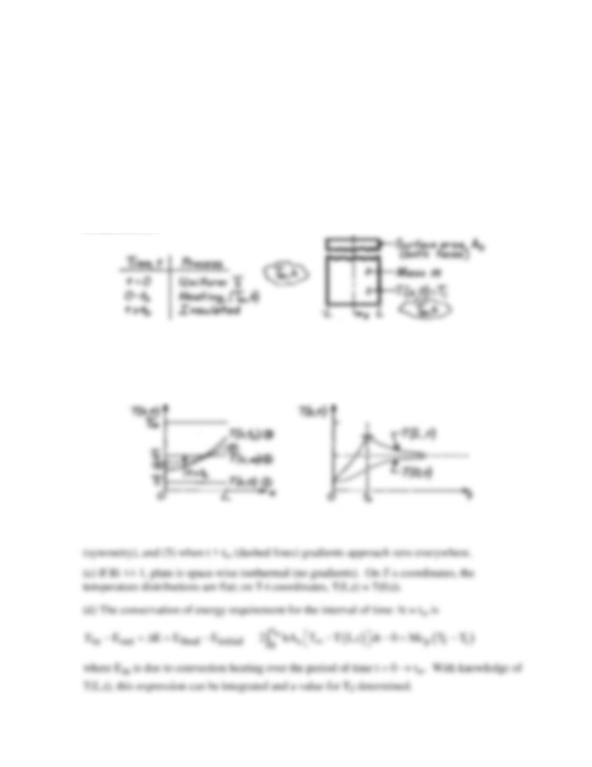
KNOWN: Stainless steel disk of known thickness, radius, emissivity, and initial temperature.
Environment and surroundings temperatures and heat transfer coefficients.
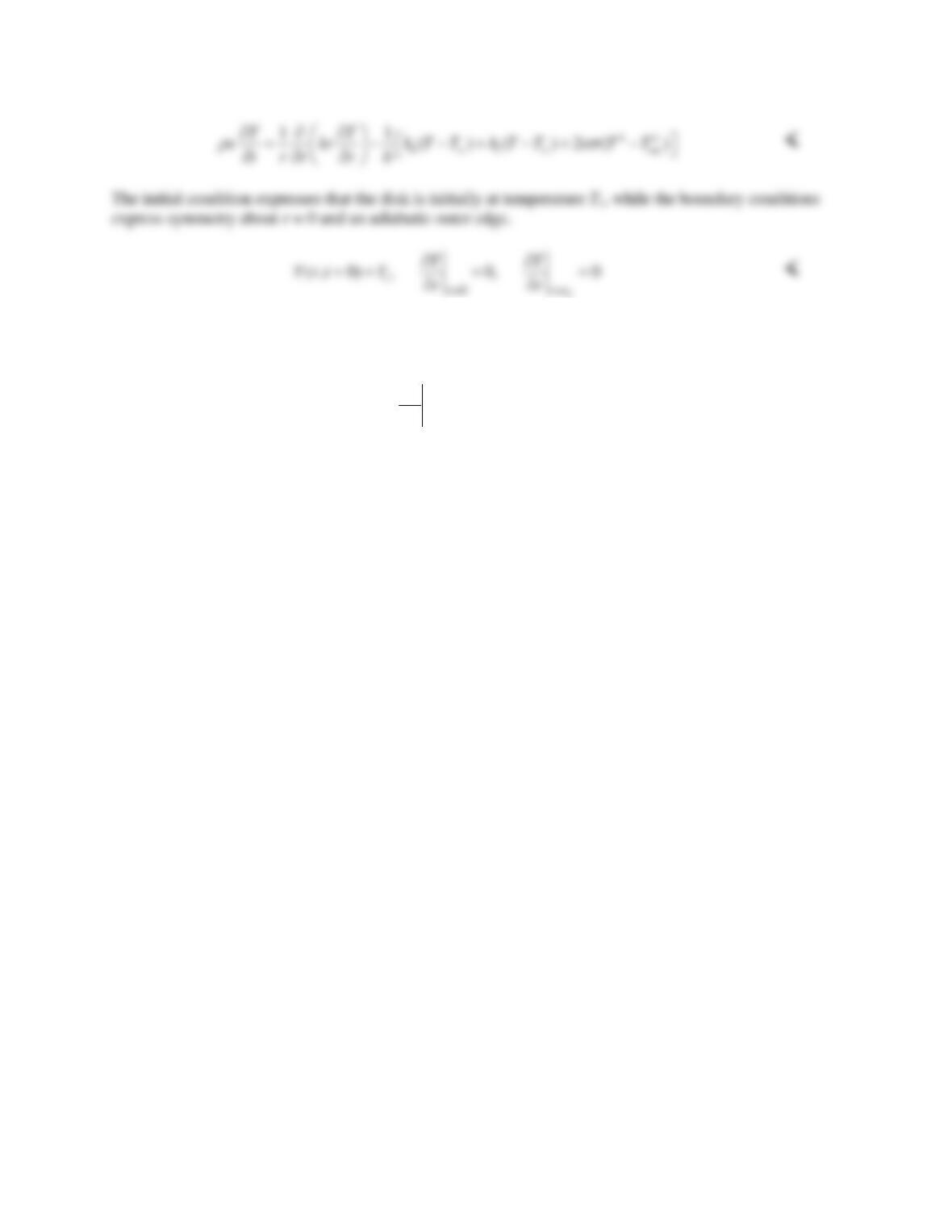
FIND: Derive differential equation governing transient temperature distribution, T(r,t). List initial and
boundary conditions.
SCHEMATIC:
ASSUMPTIONS: (1) Uniform properties. (2) Temperature is nearly uniform across the disk thickness.
(3) The surroundings are large relative to the disk. (4) Convection and radiation from the rim are
negligible because it is so thin.
ANALYSIS: Consider a differential
control volume that is a ring of width dr
where
h
t
, T
∞
PROBLEM 5.4 (Cont.)
COMMENTS: (1) The assumption of negligible temperature variation through the thickness makes this
an extended surface problem, with transient behavior. (2) The boundary condition at the outer edge could
take convection and radiation into account. Assuming a heat transfer coefficient he for the edge, the
boundary condition would become
44
sur
((,) ) ( (,) )
eo o
o
rr
T
k hTrt T T rt T
r
εs
∞
=
∂
− = −+ −
∂
.
PROBLEM 5.5
KNOWN: Plate initially at a uniform temperature Ti is suddenly subjected to convection
process (T∞,h) on both surfaces. After elapsed time to, plate is insulated on both surfaces.
FIND: (a) Assuming Bi >> 1, sketch on T – x coordinates: initial and steady–state (t → ∞)
temperature distributions, T(x,to) and distributions for two intermediate times to < t < ∞, (b)
Sketch on T – t coordinates midplane and surface temperature histories, (c) Repeat parts (a)
and (b) assuming Bi << 1, and (d) Obtain expression for T(x,∞) = Tf in terms of plate
parameters (M,cp), thermal conditions (Ti, T∞, h), surface temperature T(L,t) and heating
time to.
SCHEMATIC:
ASSUMPTIONS: (1) One-dimensional conduction, (2) Constant properties, (3) No internal
generation, (4) Plate is perfectly insulated for t > to, (5) T(0, t < to) < T∞.
ANALYSIS: (a,b) With Bi >> 1, appreciable temperature gradients exist in the plate
following exposure to the heating process.
On T-x coordinates: (1) initial, uniform temperature, (2) steady-state conditions when t → ∞,
(3) distribution at to just before plate is covered with insulation, (4) gradients are always zero
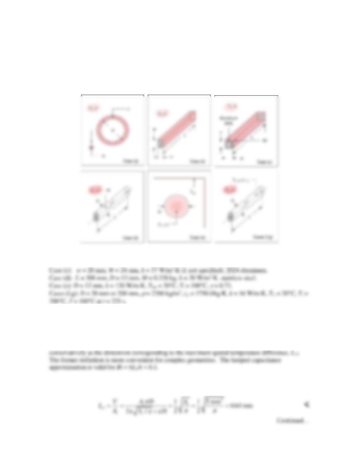
PROBLEM 5.6
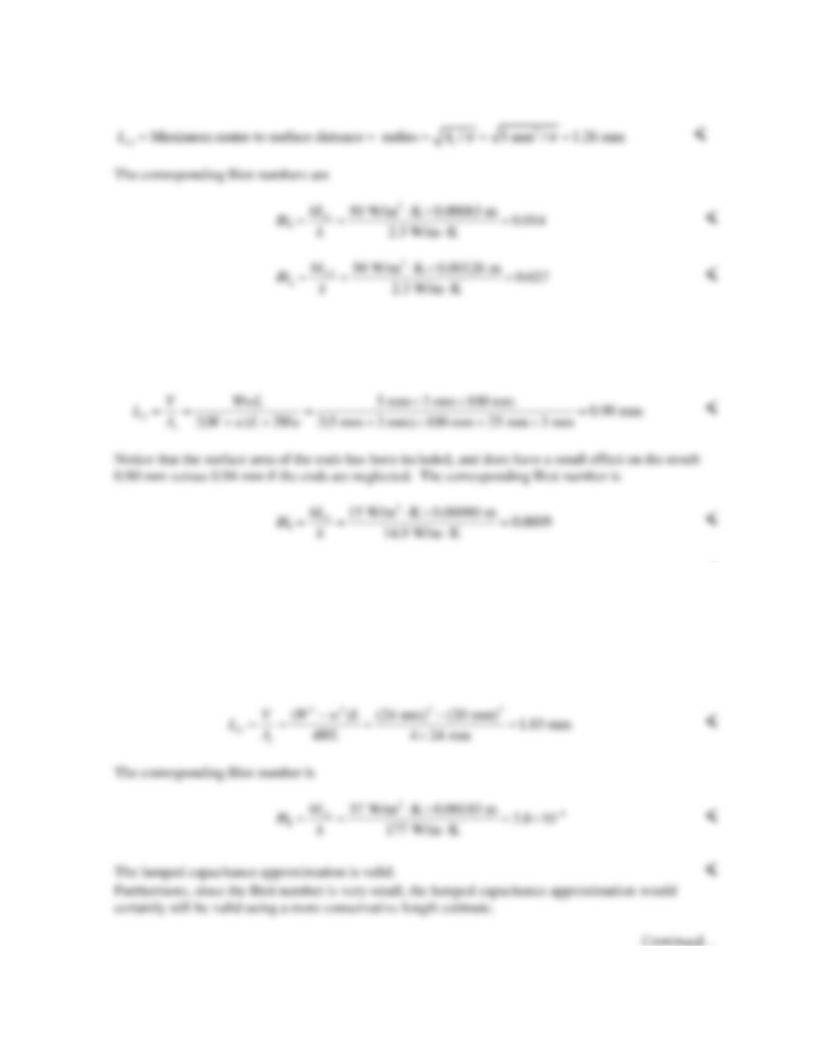
KNOWN: Geometries of various objects. Material and/or properties. Cases (a) through (d):
Convection heat transfer coefficient between object and surrounding fluid. Case (e): Emissivity of
sphere, initial temperature, and temperature of surroundings. Cases (f) and (g): Initial temperature,
spatially averaged temperature at a later time, and surrounding fluid temperature.
FIND: Characteristic length and Biot number. Validity of lumped capacitance approximation.
SCHEMATIC:
Case (a): D = 50 mm, Ac = 5 mm2, k = 2.3 W/mK, h = 50 W/m2K.
Case (b): W = 5 mm, w = 3 mm, L = 100 mm, h = 15 W/m2K, AISI 304 stainless steel.
ASSUMPTIONS: (1) Constant properties, (2) In case (e), radiation is to large surroundings.
PROPERTIES: Table A.1, Stainless steel, AISI 304 (T = 300 K): k = 14.9 W/mK. Aluminum 2024
(T = 300 K): k = 177 W/mK.
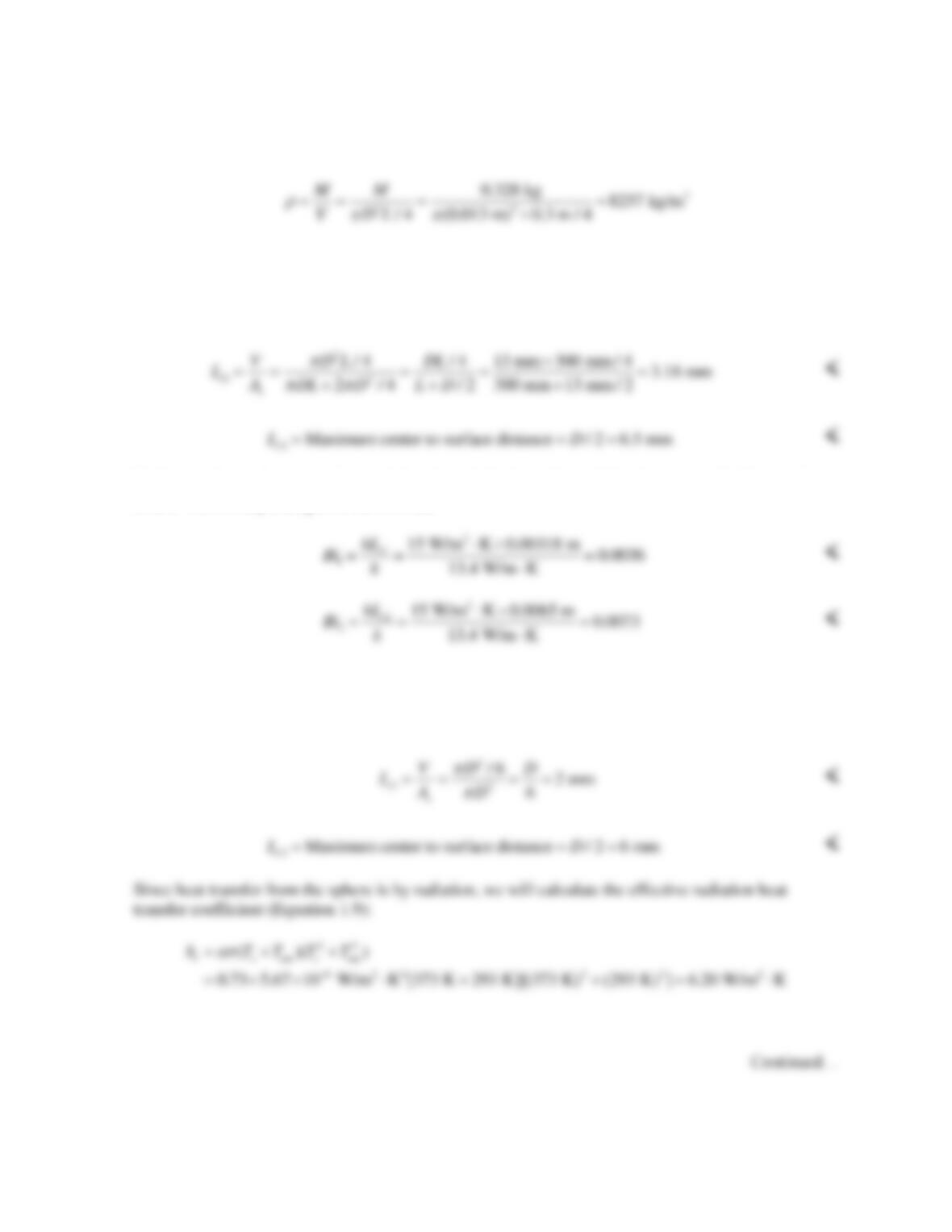
ANALYSIS: Characteristic lengths can be calculated as Lc1 = V/As, or they can be taken
(a) The radius of the torus, ro, can be found from
2
co
Ar
. The characteristic lengths are
PROBLEM 5.6 (Cont.)
The lumped capacitance approximation is valid according to either definition. <
(b) For this complex shape, we will calculate only Lc1.
The lumped capacitance approximation is valid. <
Furthermore, since the Biot number is very small, the lumped capacitance approximation would
certainly still be valid using a more conservative length estimate.
(c) Again, we will only calculate Lc1. There will be very little heat transfer to the stagnant air inside
the tube, therefore in determining the surface area for convection heat transfer, As, only the outer
surface area should be included. Thus,
Continued…
PROBLEM 5.6 (Cont.)
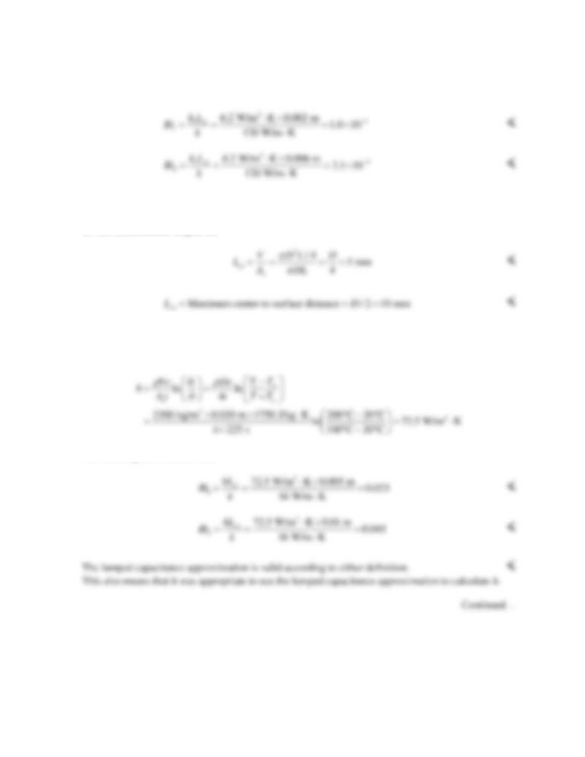
(d) We are not told which type of stainless steel this is, but we are told its mass, from which we can
find its density:
This appears to be AISI 316 stainless steel, with a thermal conductivity of k = 13.4 W/mK at T = 300
K.
The characteristic lengths are
Notice that the surface area of the ends has been included in Lc1, and does have a small effect on the
result. The corresponding Biot numbers are
The lumped capacitance approximation is valid according to either definition. <
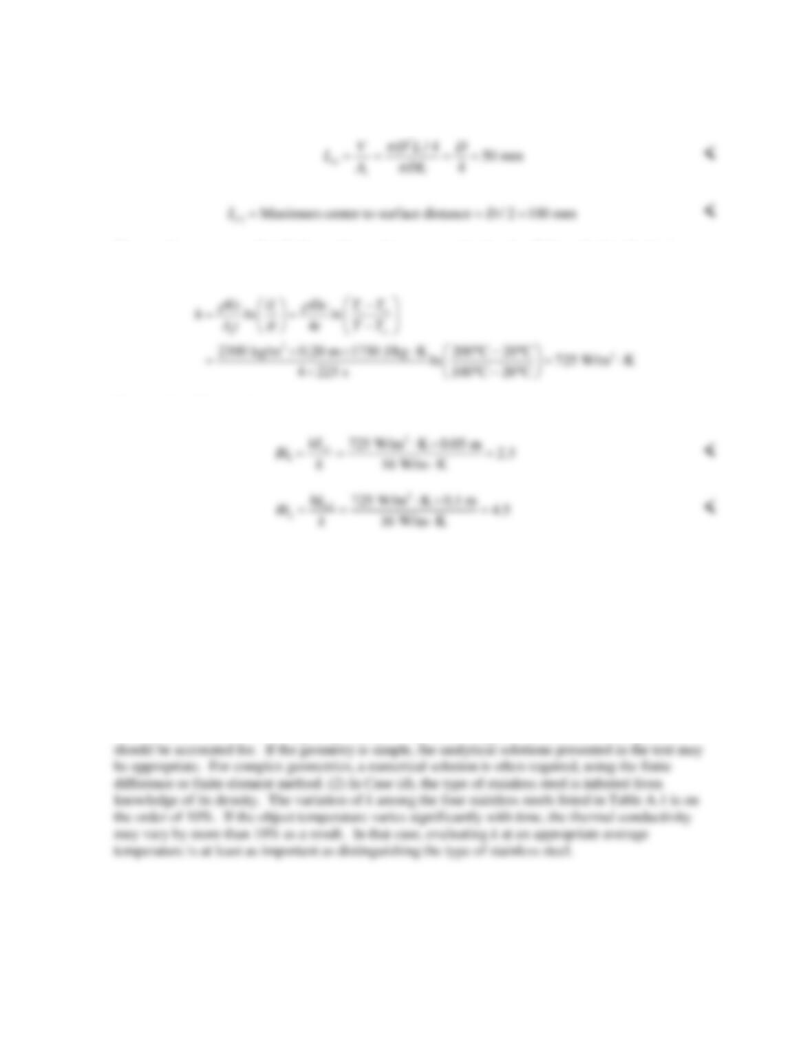
(e) The characteristic lengths are
PROBLEM 5.6 (Cont.)
The surface temperature has been taken as the initial value, to give the largest possible heat transfer
coefficient. The Biot numbers are
The lumped capacitance approximation is valid according to either definition. <
(f) The characteristic lengths are
We are not told the convection heat transfer coefficient, but we do know the fluid temperature and the
temperature of the rod initially and at t = 225 s. If we assume that the lumped capacitance
approximation is valid, we can determine the heat transfer coefficient from Equation 5.5:
The resulting Biot numbers are:
PROBLEM 5.6 (Cont.)
(g) With the diameter increased by a factor of ten, so are the characteristic lengths:
Once again, we assume that the lumped capacitance approximation is valid to calculate the heat
transfer coefficient according to
The resulting Biot numbers are:
The lumped capacitance approximation is not valid according to either definition. <
This means that the calculated value of h is incorrect, therefore the above values of the Biot number
are incorrect. However, we can still conclude that the Bi number is too large for lumped capacitance
to be valid by the following reasoning. If the lumped capacitance approximation were valid, then the
calculated h would be correct, and its value would be small enough to result in Bi < 0.1. Since the
calculated Biot number does not satisfy the criterion to use the lumped capacitance approximation, the
initial assumption that the lumped capacitance method is valid must have been false.
COMMENTS: (1) The determination of whether or not the lumped capacitance approximation can
be used is, to some degree, dependent on how much precision is required in a given application. If the
Biot number is close to 0.1 and good precision is required, the spatial variation of the temperature
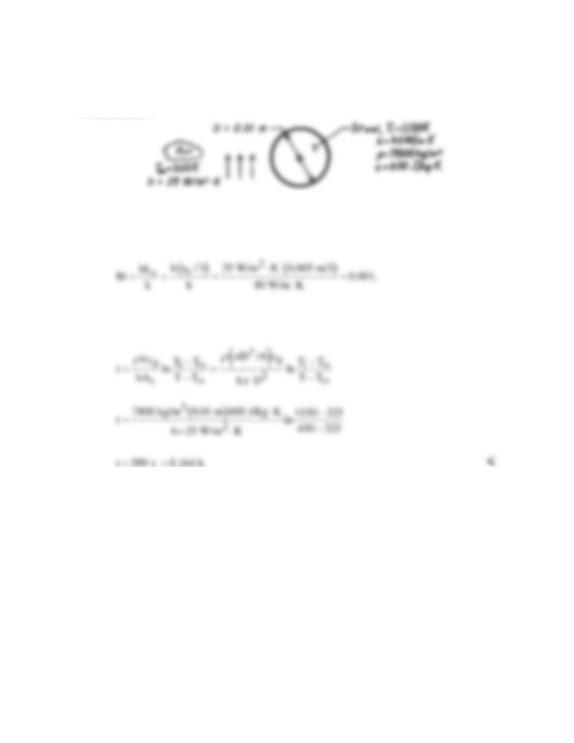
PROBLEM 5.7
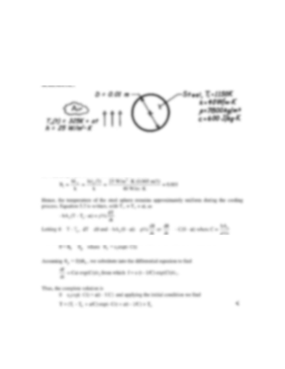
KNOWN: Diameter and initial temperature of steel balls cooling in air.
FIND: Time required to cool to a prescribed temperature.
SCHEMATIC:
ASSUMPTIONS: (1) Negligible radiation effects, (2) Constant properties.
ANALYSIS: Applying Eq. 5.10 to a sphere (Lc = ro/3),
Hence, the temperature of the steel remains approximately uniform during the cooling
process, and the lumped capacitance method may be used. From Eqs. 5.4 and 5.5,
COMMENTS: Due to the large value of Ti, radiation effects are likely to be significant
during the early portion of the transient. The effect is to shorten the cooling time.
PROBLEM 5.8
KNOWN: Diameter and initial temperature of steel balls in air. Expression for the air
temperature versus time.
FIND: (a) Expression for the sphere temperature, T(t), (b) Graph of T(t) and explanation of
special features.
ASSUMPTIONS: (1) Constant properties, (2) Negligible radiation heat transfer.
PROPERTIES: Given: k = 40 W/m∙K, ρ = 7800 kg/m3, c = 600 J/kg∙K.
ANALYSIS:
(a) Applying Equation 5.10 to a sphere (Lc = ro/3),
dt dt ρc
The solution may be written as the sum of the homogeneous and particular solutions,
Continued…
PROBLEM 5.8 (Cont.)
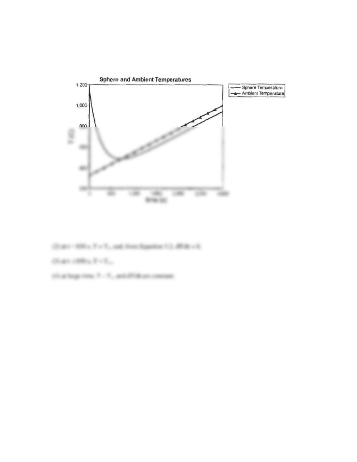
(b) The ambient and sphere temperatures for 0 ≤ t ≤ 3600 s are shown in the plot below.
Note that:
(1) For small times (t
≤
300s) the sphere temperature decreases rapidly,
COMMENTS: Unless the air environment of Problem 5.7 is cooled, the air temperature will
increase in temperature as energy is transferred from the balls. However, the actual air
temperature versus time may not be linear.
≥
PROBLEM 5.9
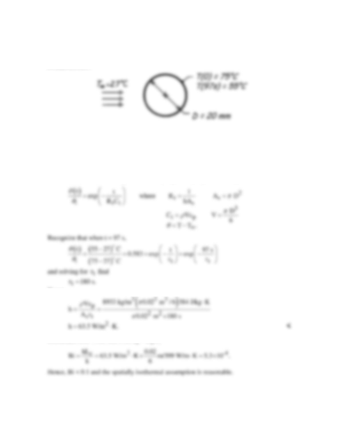
KNOWN: The temperature–time history of a pure copper sphere in a hydrogen stream.
FIND: The heat transfer coefficient between the sphere and the hydrogen stream.
SCHEMATIC:
ASSUMPTIONS: (1) Temperature of sphere is spatially uniform, (2) Negligible radiation
exchange, (3) Constant properties.
PROPERTIES: Table A-1, Pure copper (338 K): ρ = 8933 kg/m3, cp = 384 J/kg⋅K, k = 399
W/m⋅K.
ANALYSIS: The time-temperature history is given by Eq. 5.6 with Eq. 5.7.
Hence,
COMMENTS: Note that with Lc = Do/6,
PROBLEM 5.10
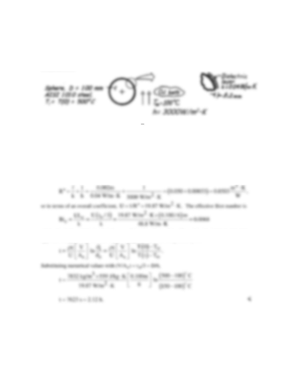
KNOWN: Solid steel sphere (AISI 1010), coated with dielectric layer of prescribed thickness and
thermal conductivity. Coated sphere, initially at uniform temperature, is suddenly quenched in an oil
bath.
FIND: Time required for sphere to reach 150°C.
SCHEMATIC:
PROPERTIES: Table A-1, AISI 1010 Steel
[ ]
( )
T 500 150 C/2 325 C 600K :=+=≈
3
7832 kg/m , c 559 J/kg K, k 48.8 W/m K.
ρ
= = ⋅= ⋅
ASSUMPTIONS: (1) Steel sphere is space–wise isothermal, (2) Dielectric layer has negligible
thermal capacitance compared to steel sphere, (3) Layer is thin compared to radius of sphere, (4)
Constant properties, (5) Neglect contact resistance between steel and coating.
ANALYSIS: The thermal resistance to heat transfer from the sphere is due to the dielectric layer and
the convection coefficient. That is,
where the characteristic length is Lc = ro/3 for the sphere. Since Bie < 0.1, the lumped capacitance
approach is applicable. Hence, Eq. 5.5 is appropriate with h replaced by U,
COMMENTS: (1) Note from calculation of
′′
R
that the resistance of the dielectric layer dominates
and therefore nearly all the temperature drop occurs across the layer.
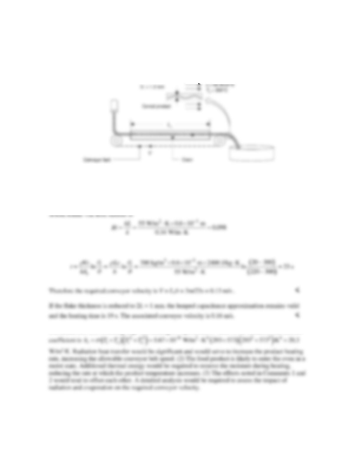
PROBLEM 5.11
KNOWN: Thickness and properties of flaked food product. Conveyor length. Initial flake
temperature. Ambient temperature and convection heat transfer coefficient. Final product temperature.
FIND: Required conveyor velocities for thick and thin flakes.
SCHEMATIC:
ASSUMPTIONS: (1) Constant properties. (2) Lumped capacitance behavior. (3) Negligible radiation
heat transfer. (4) Negligible moisture evaporation from product. (5) Negligible conduction between
flake and conveyor belt.
PROPERTIES: Flake:
= 700 kg/m3, cp = 2400 J/kgK, and k = 0.34 W/mK.
Hence the lumped capacitance assumption is valid. The required heating time is
COMMENTS: (1) Assuming large surroundings, a representative value of the radiation heat transfer
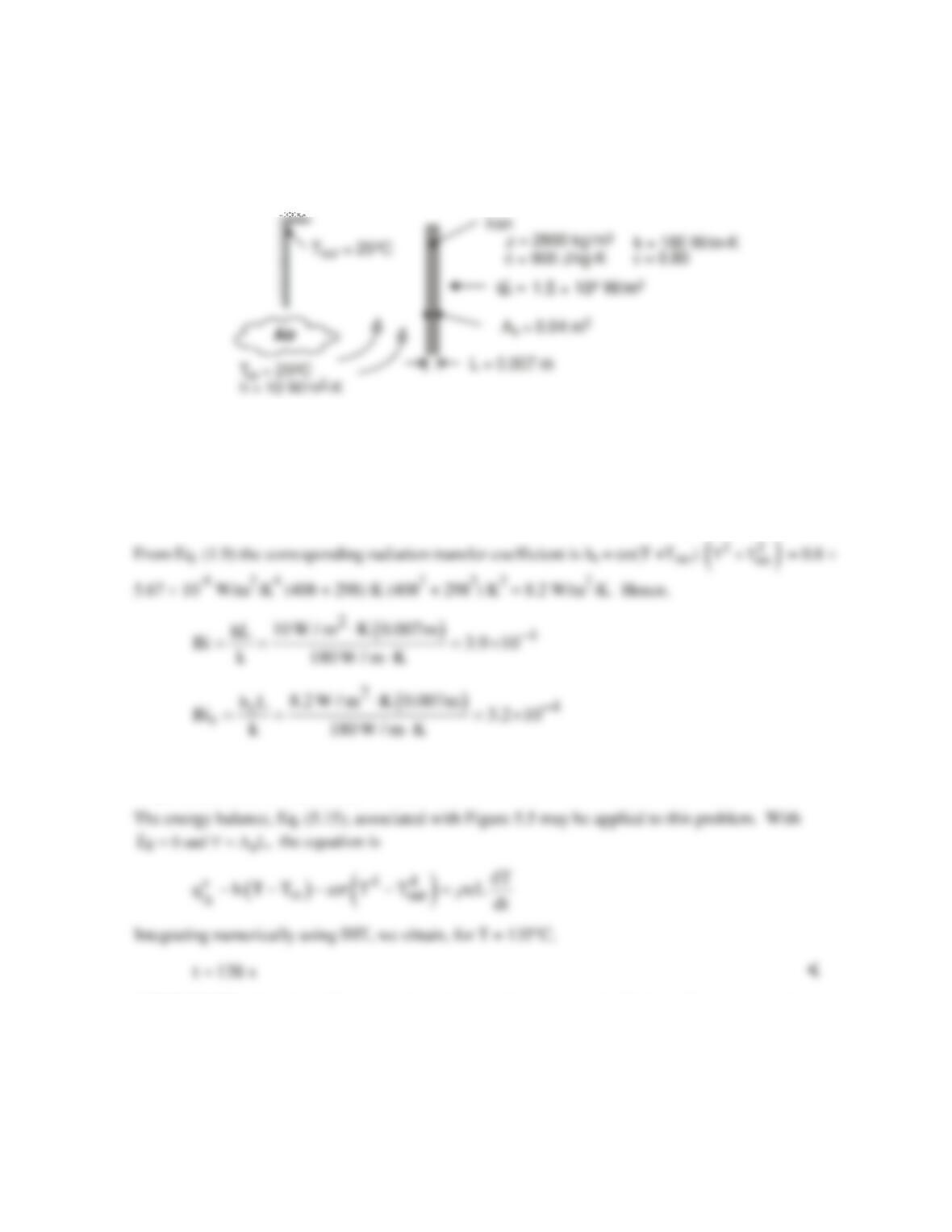
PROBLEM 5.12
KNOWN: Thickness, surface area, and properties of iron base plate. Heat flux at inner surface.
Temperature of surroundings. Temperature and convection coefficient of air at outer surface.
FIND: Time required for plate to reach a temperature of 135°C. Operating efficiency of iron.
SCHEMATIC:
ASSUMPTIONS: (1) Radiation exchange is between a small surface and large surroundings, (2)
Convection coefficient is independent of time, (3) Constant properties, (4) Iron is initially at room
temperature (Ti = T∞).
ANALYSIS: Biot numbers may be based on convection heat transfer and/or the maximum heat
transfer by radiation, which would occur when the plate reaches the desired temperature (T = 135°C).
With convection and radiation considered independently or collectively, Bi, Bir, Bi + Bir << 1 and the
lumped capacitance analysis may be used.
COMMENTS: Note that, if heat transfer is by natural convection, h, like hr, will vary during the
process from a value of 0 at t = 0 to a maximum at t = 138 s.
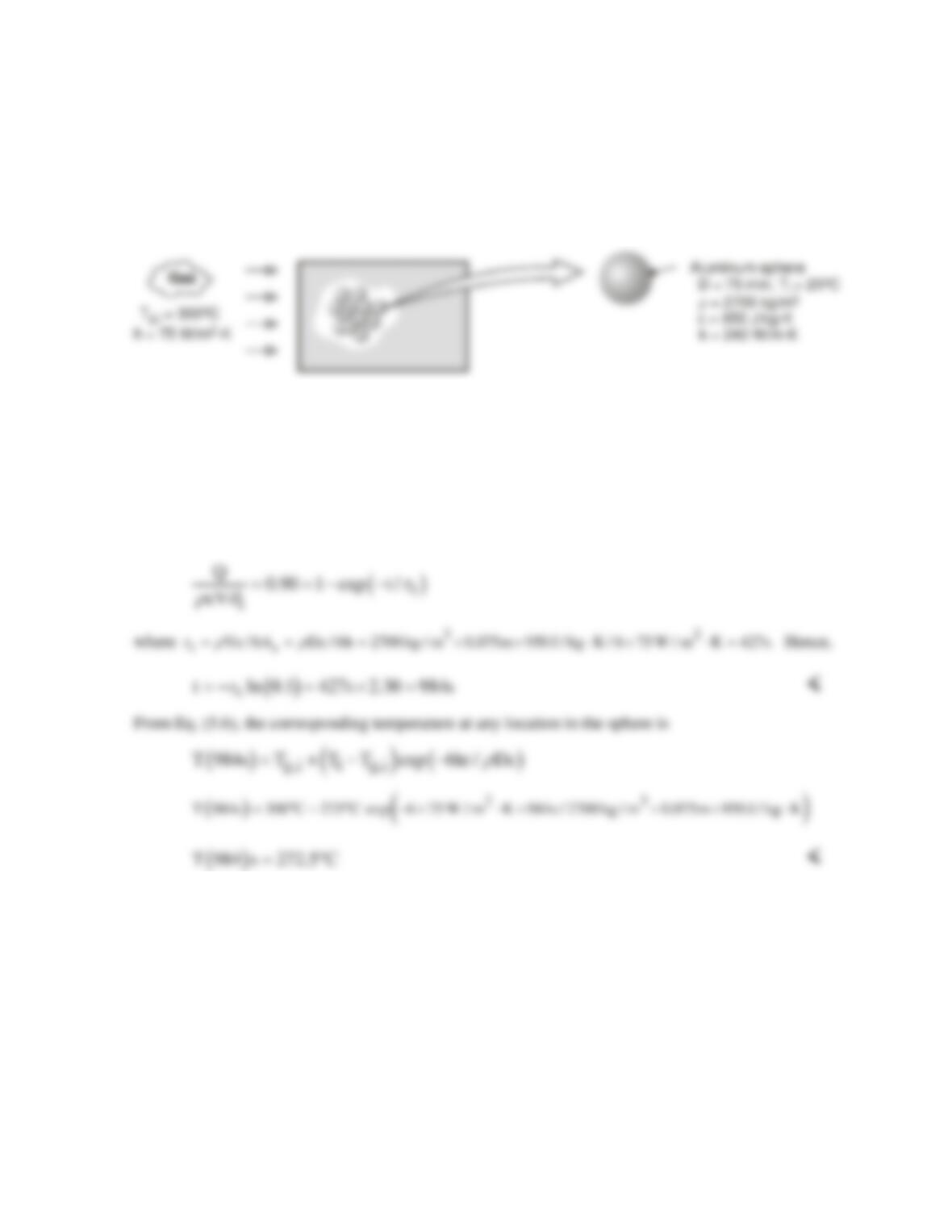
PROBLEM 5.13
KNOWN: Diameter, density, specific heat and thermal conductivity of aluminum spheres used in
packed bed thermal energy storage system. Convection coefficient and inlet gas temperature.
FIND: Time required for sphere to acquire 90% of maximum possible thermal energy and the
corresponding center temperature. Potential advantage of using copper in lieu of aluminum.
SCHEMATIC:
ASSUMPTIONS: (1) Negligible heat transfer to or from a sphere by radiation or conduction due to
contact with other spheres, (2) Constant properties.
ANALYSIS: To determine whether a lumped capacitance analysis can be used, first compute Bi =
h(ro/3)/k = 75 W/m2⋅K (0.0125 m)/240 W/m⋅K = 0.0039 < 0.1. Hence, the lumped capacitance
approximation may be made, and a uniform temperature may be assumed to exist in the sphere at any
time. From Eq. 5.8a, achievement of 90% of the maximum possible thermal energy storage
corresponds to
Obtaining the density and specific heat of copper from Table A-1, we see that (ρc)Cu ≈ 8900 kg/m3 ×
400 J/kg⋅K = 3.56 × 10⁶ J/m3⋅K > (ρc)Al = 2.57 × 10⁶ J/m3⋅K. Hence, for an equivalent sphere
diameter, the copper can store approximately 38% more thermal energy than the aluminum.
COMMENTS: Before the packed bed becomes fully charged, the temperature of the gas decreases
as it passes through the bed. Hence, the time required for a sphere to reach a prescribed state of
thermal energy storage increases with increasing distance from the bed inlet.
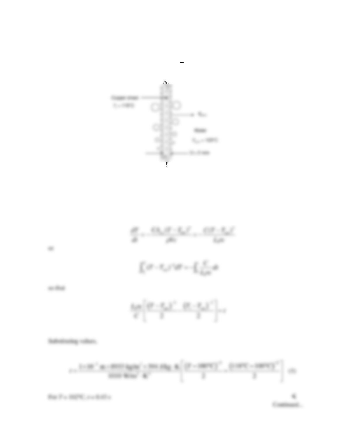
PROBLEM 5.14
KNOWN: Thickness and initial temperature of copper sheet. Dependence of the convection heat
transfer coefficient on sheet temperature.
FIND: Time required to reach sheet temperature of
T
= 102°C.
SCHEMATIC:
ASSUMPTIONS: (1) Constant properties. (2) Lumped capacitance behavior.
PROPERTIES: Table A.1, copper (T = 383 K):
ρ
= 8933 kg/m3, c = 394 J/kg⋅K, and k = 394 W/m⋅K.
ANALYSIS: Since h = 1010 W/m2⋅K3(T – Tsat)2 the values of C and n in Equation 5.26 are 1010
W/m2∙K3 and 2, respectively. Equation 5.27 becomes