Chapter 5 representing a rotation or a reflection

Section 5.3

5.3.32 a No! As a counterexample, consider A=



1 0

0 1

0 0



(see Exercise 30).

b Yes! More generally, if Aand Bare n×nmatrices such that BA =In, then AB =In, by Theorem 2.4.8c.

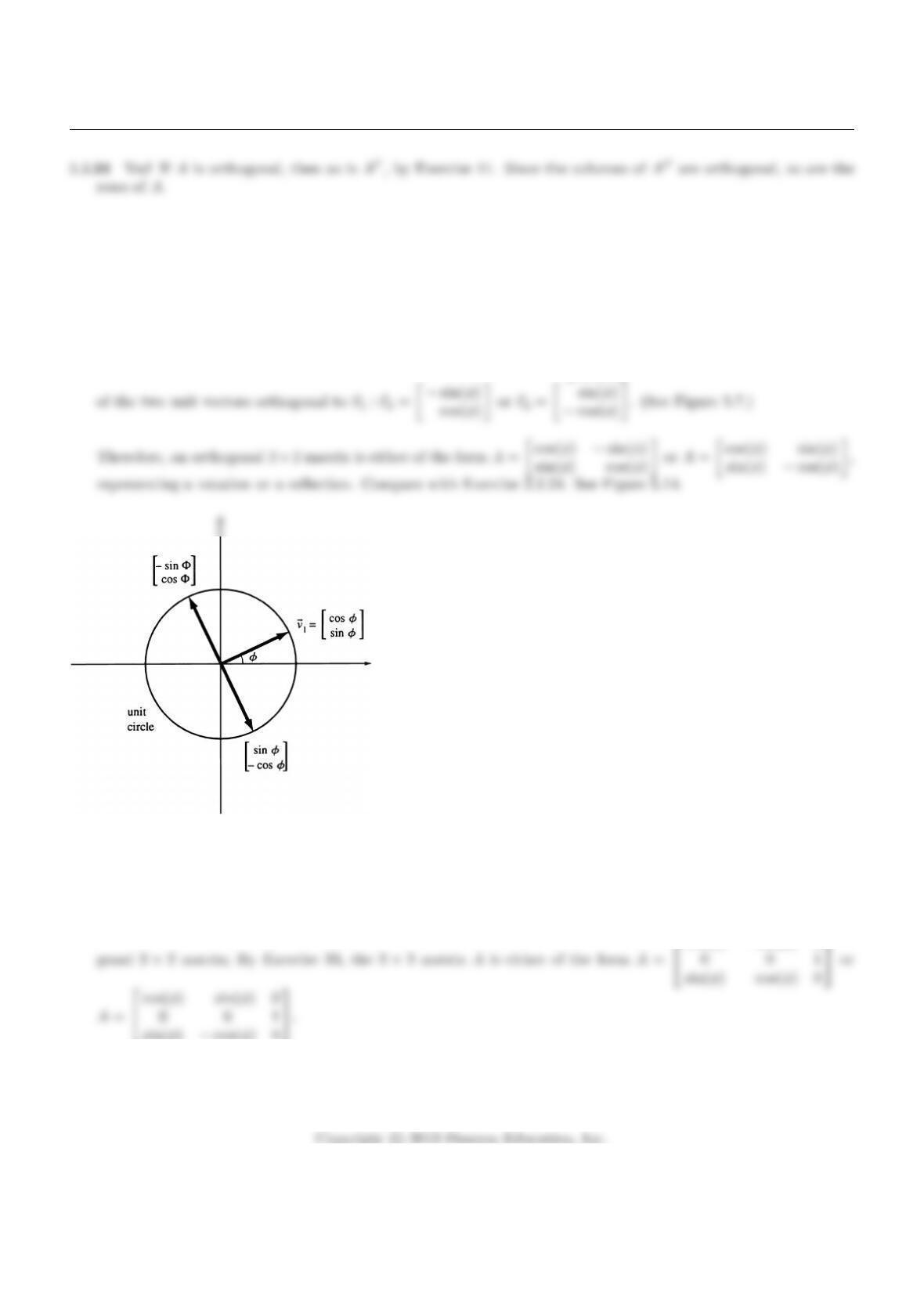
5.3.33 Write A= [ ~v1~v2]. The unit vector ~v1can be expressed as ~v =cos(φ)

sin(φ), for some φ. Then ~v2will be one

Figure 5.14: for Problem 5.3.33.

5.3.34 Since the first two columns are orthogonal to the third, we have c=d= 0. Then a b

e f is an ortho-

cos(φ)−sin(φ) 0



5.3.35 Let us first think about the inverse L=T−1of T.

247

Chapter 5

Write L(~x) = A~x = [ ~v1~v2~v3]~x. It is required that L(~e3) = ~v3=



2

3

2

3

1

3



.

−2



5.3.36 Let the third column be the cross product of the first two: A=





2

3

1

√2

1

√18

2

3−1

√2

1

√18

1

30−4

√18





.

5.3.38 a The general form of a skew-symmetric 3 ×3 matrix is A=



0a b

−a0c

−b−c0



, with

A2=

−a2−b2−bc ac

−bc −a2−c2−ab

ac −ab −b2−c2

, a symmetric matrix.

b By Theorem 5.3.9.a, (A2)T= (AT)2= (−A)2=A2, so that A2is symmetric.

5.3.39 By Theorem 5.3.10, the matrix of the projection is ~u~uT; the ij th entry of this matrix is uiuj.

Section 5.3

5.3.41 A unit vector on the line is ~u =1

√n



1

.

1



.

The matrix of the orthogonal projection is ~u~uT, the n×nmatrix whose entries are all 1

n(compare with Exer-

cise 39).

5.3.42 a Suppose we are projecting onto a subspace Wof Rn. Since A~x is in Walready, the orthogonal projection

of A~x onto Wis just A~x itself: A(A~x) = A~x, or A2~x =A~x.

5.3.43 Examine how Aacts on ~u, and on a vector ~v orthogonal to ~u:

A~u = (2~u~uT−I3)~u = 2~u~uT~u −~u =~u, since ~uT~u =~u ·~u =k~uk2= 1.

5.3.44 Note that ATis an m×nmatrix. By Theorems 3.3.7 and 5.3.9c we have

5.3.45 Note that ATis an m×nmatrix. By Theorems 3.3.7 and 5.3.9c, we have

5.3.46 By Theorem 5.2.2, the columns ~u1, . . . , ~umof Qare orthonormal. Therefore, QTQ=Im, since the ij th entry

5.3.47 By Theorem 5.2.2, the columns ~u1, . . . , ~umof Qare orthonormal. Therefore, QTQ=Im, since the ij th entry

of QTQis ~ui·~uj.

By Theorem 5.3.9a, we now have ATA= (QR)TQR =RTQTQR =RTR.

249

Chapter 5

5.3.48 As suggested, we consider the QR factorization

AT=P R

5.3.49 Yes! By Exercise 5.2.45, we can write AT=P L, where Pis orthogonal and Lis lower triangular.

5.3.50 a If an n×nmatrix Ais orthogonal and upper triangular, then A−1is both lower triangular (since A−1=AT)

and upper triangular (being the inverse of an upper triangular matrix; compare with Exercise 2.4.35c).

Therefore, A−1=ATis a diagonal matrix, and so is Aitself. Since Ais orthogonal with positive diagonal entries,

5.3.51 a Using the terminology suggested in the hint, we observe that Im=QT

1Q1= (Q2S)TQ2S=STQT

2Q2S=

STS, so that Sis orthogonal, by Theorem 5.3.7.

5.3.52 Applying the strategy outlined in Summary 4.1.6 to the general element 



a b c

b d e



of V, we find the basis

5.3.53 Applying the strategy outlined in Summary 4.1.6 to the general element 



0b c

−b0e

−c−e0



of V, we find the

5.3.54 To write the general form of a skew-symmetric n×nmatrix A, we can place arbitrary constants above the

diagonal, the opposite entries below the diagonal (aij =−aji), and zeros on the diagonal (since aii =−aii). See

Exercise 53 for the case n= 3. Thus the dimension of the space equals the number of entries above the diagonal

of an n×nmatrix. In Exercise 55 we will see that there are (n2−n)/2 such entries. Thus dim(V) = (n2−n)/2.

250

Section 5.3

5.3.55 To write the general form of a symmetric n×nmatrix A, we can place arbitrary constants on and above

the diagonal, and then write the corresponding entries below the diagonal (aij =aji). See Exercise 52 for the

5.3.56 Yes and yes (see Exercise 57).

5.3.57 Yes, Lis linear, since L(A+B) = (A+B)T=AT+BT=L(A)+L(B) and L(kA) = (kA)T=kAT=kL(A).

Yes, Lis an isomorphism; the inverse is the transformation R(A) = ATfrom Rn×mto Rm×n.

5.3.59 The kernel consists of all matrixes Asuch that L(A) = 1

2(A−AT) = 0, that is, AT=A; those are the

symmetric matrices.

5.3.60 Using Theorem 4.3.2, we find the matrix 





1 0 0 0

0 1 0 0

0 0 1 0

0 0 0 −1





.

5.3.61 Note that the first three matrices of the given basis Bare symmetric, so that L(A) = A−AT= 0, and the

coordinate vector [L(A)]Bis ~

0 for all three of them. The last matrix of the basis is skew-symmetric, so that



5.3.63 By Exercise 2.4.94b, the given LDU factorization of Ais unique.

5.3.64 aA−BT

B AT+C−DT

D CT=A+C−BT−DT

B+D AT+CT

=A+C−(B+D)T

B+D(A+C)Tis of the required form.

251

Chapter 5

bkA−BT

B AT=kA −kBT

kB kAT=kA −(kB)T

kB (kA)Tis of the required form.

eA−BT

B ATT

=ATBT

−B(AT)Tis of the required form.

f Note that the columns ~v1, ~v2, ~v3, ~v4or Mare orthogonal, and they all have length pp2+q2+r2+s2. Now

MTMis the 4 ×4 matrix whose ij th entry is ~vi·~vj, so that MTM= (p2+q2+r2+s2)I4.

5.3.65 Write 10A=a b

c d ; it is required that a, b, c and dbe integers. Now A=a

10

b

10

c

10

d

10 must be an orthogonal

matrix, implying that ( a

5.3.66 One approach is to take one of the solutions from Exercise 65, say, the rotation matrix B=0.8−0.6

0.6 0.8,

and then let A=B2=0.28 −0.96

0.96 0.28 . Matrix Ais orthogonal by Theorems 5.3.4a.

252

Section 5.3

5.3.68 If A=QR, then A(ATA)−1AT=QR(RTQTQR)−1RTQT=QR(RTR)−1RTQT=QRR−1(RT)−1RTQT=

QQT,as in Theorem 5.3.10. The equation QTQ=Imholds since the columns of Qare orthonormal.

5.3.69 We will use the terminology introduced in Theorem 5.3.10. Since the two given vectors ~v1and ~v2are

orthogonal (verify that ~v1·~v2= 0), with k~v1k=k~v2k=√3, we have the orthonormal basis ~u1=1

√3~v1, ~u2=1

√3~v2

, so

5.3.70 a. We will use the terminology introduced in Theorem 5.3.10. Consider the basis B= (~v1, ~v2) of Vpresented

in Exercise 4.3.73c. Since the two vectors ~v1and ~v2are orthogonal (verify that ~v1·~v2= 0), with k~v1k=k~v2k=√6,

we have the orthonormal basis ~u1=1

√6~v1, ~u2=1

√6~v2, so

Q=1

√6







0 2

1−1

1 1

2 0







and PV=QQT=1

6







0 2

1−1

1 1

2 0





0 1 1 2

2−110=1

6







4−2 2 0

−2 2 0 2

2 0 2 2

0 2 2 4







.



5.3.71 If Aand Bare Hankel matrices of size n×n, and C=A+B, then cij =aij +bij =ai+1,j−1+bi+1,j−1=

ci+1,j−1for all i= 1, …, n −1 and for all j= 2, …, n, showing that Cis a Hankel matrix as well. An analogous

argument shows that the Hankel matrices are closed under scalar multiplication.

Now, what is the dimension of the space Hnof the Hankel matrices of size n×n? In the case n= 4, the dimension

Chapter 5

5.3.72 We will use the terminology introduced in Theorem 5.3.10. Let

Q=~u =1

k~vk~v =1

k~vk







1

a

a2

…







and P=QQT=1

k~vk2







1a a2… an−1

a a2a3… an

a2a3a4… an+1

… … … … …







,

5.3.73 a. Note that ab =(1+√5)(1−√5)

4=−1. Now

~a ·~

b= 1 + ab + (ab)2+ (ab)3+… + (ab)n−2+ (ab)n−1= 1 −1 + 1 −1 + … + 1 −1 = 0,

5.3.74 a.

m-5 -4 -3 -2 -1 0 1 2 3 4 5

fm5 -3 2 -1 1 0 1 1 2 3 5

b. We conjecture that fm=f−mfor odd mand fm=−f−mfor even m.

We will prove this conjecture by induction, with the base case, f1=f−1, being established in the table above.

Assuming the result for positive integers < m, we will prove it for m.

254

Section 5.4

Since Pis a Hankel matrix, it is determined by its first and last columns, so that Phas the form given in the

exercise.

f. Using the result k~vk2=k~wk2= 40 = 5 ·8 = f5f6from part c, we find

Section 5.4

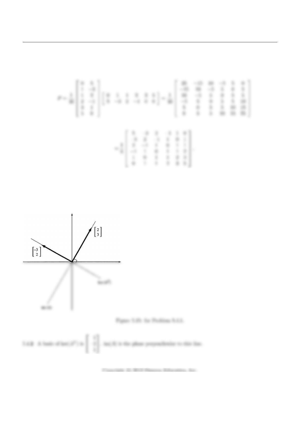
5.4.1A basis of ker(AT) is −3

2. (See Figure 5.15.)

255

Chapter 5

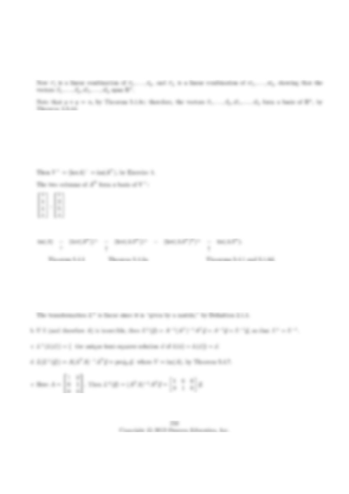
5.4.3We will first show that the vectors ~v1, . . . ,~vp, ~w1, . . . , ~wqspan Rn. Any vector ~v in Rncan be written as

~v =~vk+~v⊥, where ~vkis in Vand ~v⊥is in V⊥(by definition of orthogonal projection, Theorem 5.1.4).

5.4.4By Theorem 5.4.1, the equation (im B)⊥= ker(BT) holds for any matrix B. Now let B=AT. Then

(im(AT))⊥= ker(A). Taking transposes of both sides and using Theorem 5.1.8d we obtain im(AT) = (kerA)⊥,

as claimed.

5.4.5V= ker(A), where A=1 1 1 1

1 2 5 4 .

5.4.6Yes! For any matrix A,

5.4.7im(A) and ker(A) are orthogonal complements by Theorem 5.4.1:

(imA)⊥= ker(AT) = ker(A)

5.4.8a By Theorem 5.4.6, L+(~y) = (ATA)−1AT~y.

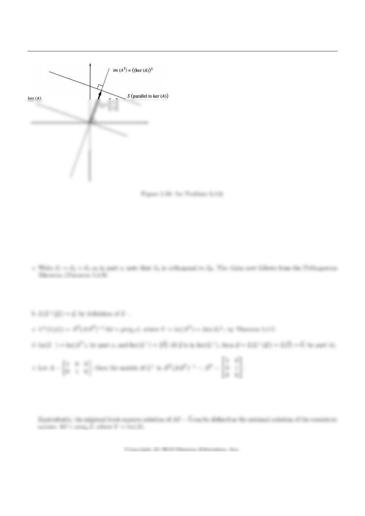
5.4.9~x0is the shortest of all the vectors in S. (See Figure 5.16.)

Section 5.4

5.4.10 a If ~x is an arbitrary solution of the system A~x =~

b, let ~xh= projV~x, where V= ker(A), and ~x0=~x−projV~x.

Note that ~

b=A~x =A(~xh+~x0) = A~xh+A~x0=A~x0, since ~xhis in ker(A).

b If ~x0and ~x1are two solutions of the system A~x =~

b, both from (kerA)⊥, then ~x1−~x0is in the subspace (kerA)⊥

as well. Also, A(~x1−~x0) = A~x1−A~x0=~

b−~

b=~

0, so that ~x1−~x0is in ker(A). By Theorem 5.1.8b, it follows

that ~x1−~x0=~

0, or ~x1=~x0, as claimed.

5.4.11 a Note that L+(~y) = AT(AAT)−1~y; indeed, this vector is in im(AT) = (kerA)⊥, and it is a solution of

L(~x) = A~x =~y.

5.4.12 By Theorem 5.4.5, the least-squares solutions of the linear system A~x =~

bare the exact solutions of the

(consistent) system ATA~x =AT~

b. The minimal solution of this normal equation (in the sense of Exercise 10) is

called the minimal least-squares solution of the system A~x =~

b.

257

Chapter 5

5.4.13 a Suppose that L+(~y1) = ~x1and L+(~y2) = ~x2; this means that ~x1and ~x2are both in (kerA)⊥= im(AT), ATA~x1=

AT~y1, and ATA~x2=AT~y2. Then ~x1+~x2is in im(AT) as well, and ATA(~x1+~x2) = AT(~y1+~y2), so that

L+(~y1+~y2) = ~x1+~x2.

The verification of the property L+(k~y) = kL+(~y) is analogous.

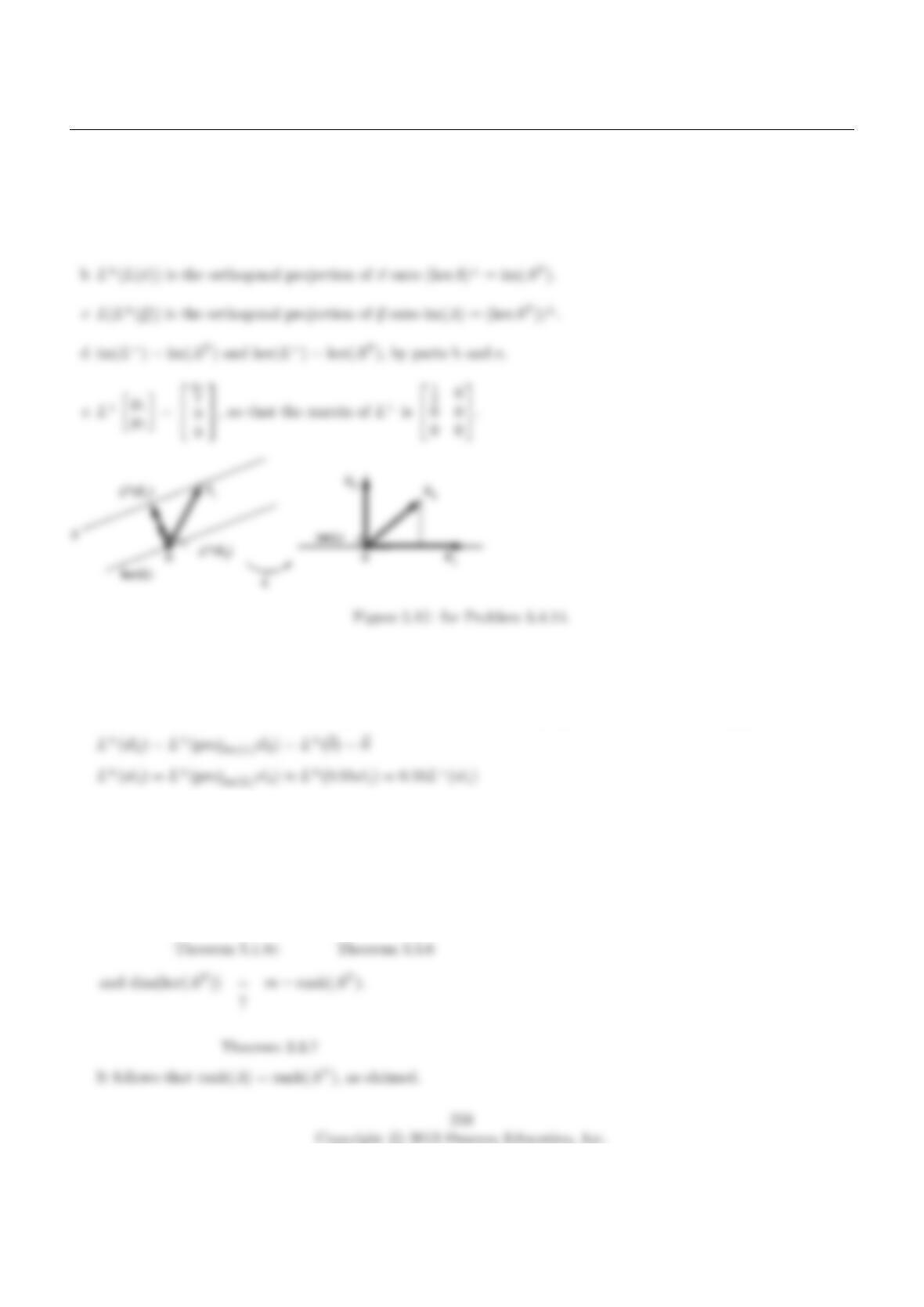
5.4.14 L+(~w1) is the minimal solution of the system L(~x) = ~w1. The line Sin Figure 5.17 shows all solutions of

the system

L(~x) = ~w1(compare with Exercise 9). The minimal solution, L+(~w1), is perpendicular to ker(L).

5.4.15 Note that (ATA)−1ATA=In; let B= (ATA)−1AT.

5.4.16 If Ais an m×nmatrix, then

dim(imA)⊥=m−dim(imA) = m−rank(A)

↑ ↑

Section 5.4

5.4.17 Yes! By Theorem 5.4.2, ker(A) = ker(ATA). Taking dimensions of both sides and using Theorem 3.3.7, we

find that n−rank(A) = n−rank(ATA); the claim follows.

5.4.19 ~x∗= (ATA)−1AT~

b=1

1, by Theorem 5.4.6.

5.4.21 Using Theorem 5.4.6, we find ~x∗=−1

2and ~

b−A~x∗=

−12

36

−18



, so that k~

b−A~x∗k= 42.

5.4.25 In this case, the normal equation ATA~x =AT~

bis 5 15

15 45 x1

x2=5

15 , which simplifies to x1+ 3x2= 1,

or x1= 1 −3x2. The solutions are of the form ~x∗=1−3t

t, where tis an arbitrary constant.

5.4.27 The least-squares solutions of the system SA~x =S~

bare the exact solutions of the normal equation (SA)TSA~x =

(SA)TS~

b.

5.4.28 The least-squares solutions of the system A~x =~unare the exact solutions of A~x = projim(A)~un. Note that

~unis orthogonal to im(A), so that projim(A)~un=~

0, and the unique least-squares solution is ~x∗=~

0.

259

Chapter 5

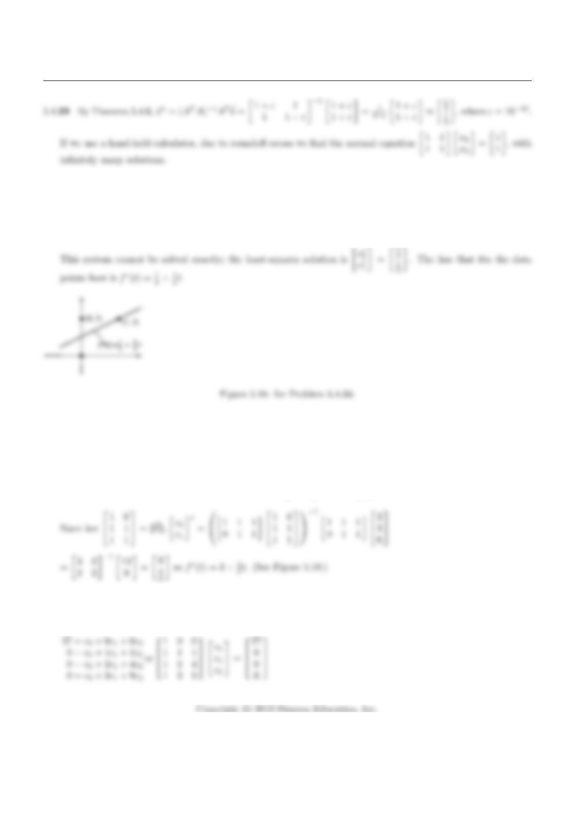
5.4.30 We attempt to solve the system

c0+ 0c1= 0

c0+ 0c1= 1

c0+ 1c1= 1

,or 



1 0

1 1



c0

c1=



0

1



.

The line goes through the point (1, 1) and “splits the diﬀerence” between (0, 0) and (0, 1). See Figure 5.18.

5.4.31 We want c0

c1such that

3 = c0+ 0c1

3 = c0+ 1c1

6 = c0+ 1c1

or 



1 0

1 1



c1

c2=



3

6



.

5.4.32 We want 



c0

c1

c2



of f(t) = c0+c1t+c2t2such that

260

Section 5.4

5.4.33 We want 



c0

c1

c2



such that

5.4.34 We want 





c0

c1

c2

c3

c4







such that

261

Chapter 5

c4

0.043

5.4.35 a The ij th entry of AT

nAnis the dot product of the ith row of AT

nand the jth column of An, i.e.

AT

nAn=







n

X

i=1

sin ai

n

X

i=1

cos ai

n

X

i=1

sin ai

n

X

i=1

sin2ai

n

X

i=1

sin aicos ai

n

X

i=1

cos ai

n

X

i=1

sin aicos ai

n

X

i=1

cos2ai







and AT

n~

b=







n

X

i=1

g(ai)

n

X

i=1

g(ai) sin ai

n

X

i=1

g(ai) cos ai







.

(Here 2π

n= ∆tso lim

n→∞

2π

n

X

i=1

cos(ti) = lim

n→∞

n

X

i=1

cos(ti)∆t=Z2π

0

cos t dt for instance.

All other limits are obtained similarly. )

262