PROBLEM 5.107 (Cont.)
Using finite–difference equations (14-16) with Eq. (13), the calculations may be performed to obtain
p
t(s)
T1
T2
T3
T4
T5
T6
T7
T8
T9
T10(°C)
0
0
200
200
200
200
200
200
200
200
200
200
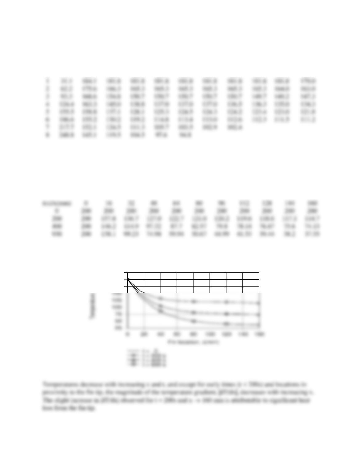
Using linear interpolation between rows 7 and 8, we obtain T(L/2, 230s) = T5 ≈ 100°C. <
(b) Using the option concerning Finite-Difference Equations for One–Dimensional Transient
Conduction in Extended Surfaces from the IHT Toolpad, the desired temperature histories were
computed for 0 ≤ t ≤ t1 = 930s. A Lookup Table involving data for T(x) at t = 0, 200, 400 and 930s was
created.
87.7
79.8
75.6
38.2
and the LOOKUPVAL2 interpolating function was used with the Explore and Graph feature of IHT to
create the desired plot.
175
200
225
COMMENTS: The steady-state condition may be obtained by extending the finite-difference
calculations in time to t ≈ 2650s or from Eq. 3.75.
1
2
3
4
5
6
7
8
PROBLEM 5.108
KNOWN: Tantalum rod initially at a uniform temperature, 300K, is suddenly subjected to a
current flow of 80A; surroundings (vacuum enclosure) and electrodes maintained at 300K.
FIND: (a) Estimate time required for mid-length to reach 1000K, (b) Determine the steady–
state temperature distribution and estimate how long it will take to reach steady–state. Use a
finite–difference method with a space increment of 10mm.
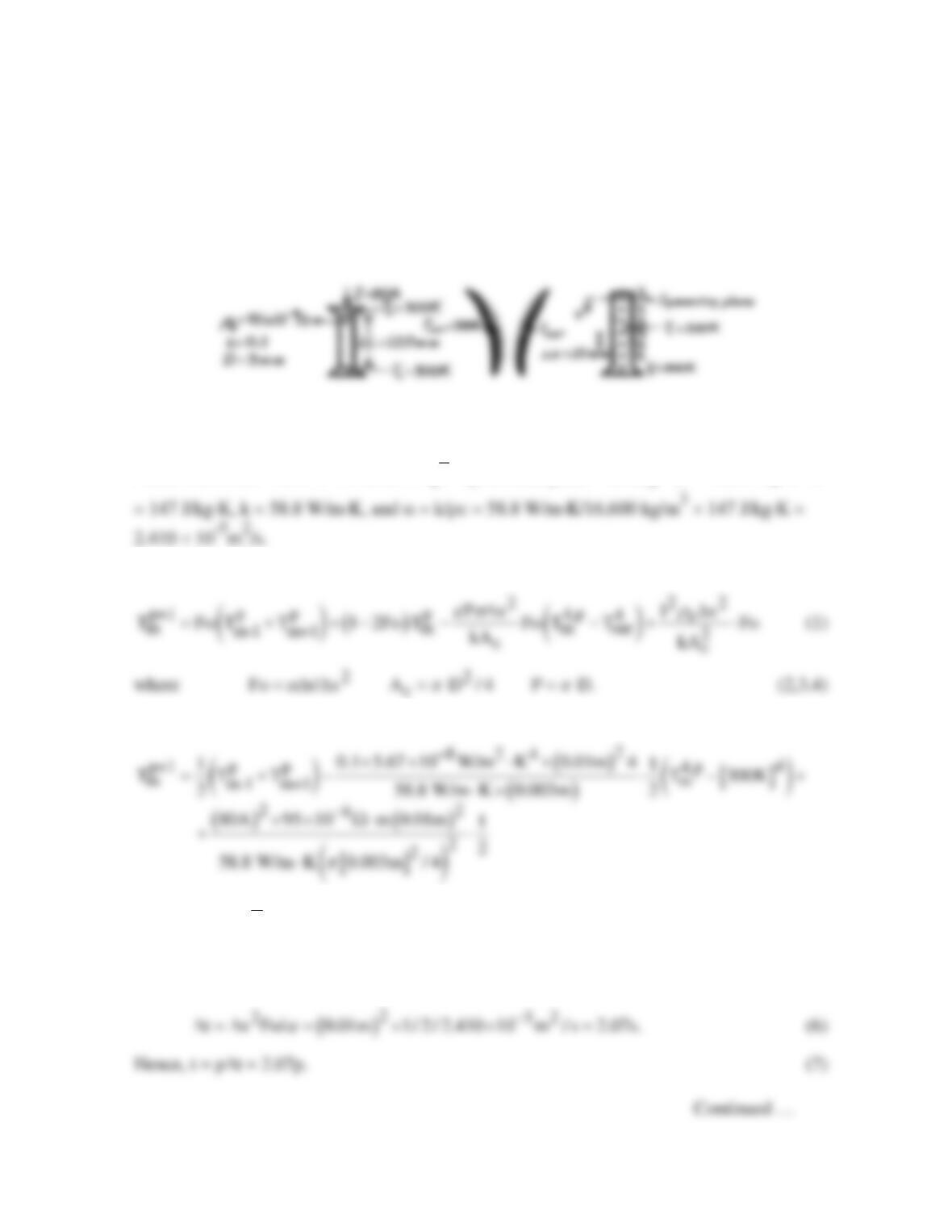
SCHEMATIC:
ASSUMPTIONS: (1) One-dimensional, transient conduction in rod, (2) Surroundings are
much larger than rod, (3) Properties are constant and evaluated at an average temperature.
PROPERTIES: Table A-1, Tantalum
( )
( )
T 300+1000 K/2 650K := =
ρ = 16,600 kg/m3, c
ANALYSIS: The finite–difference equation is
From the stability criterion, let Fo = 1/2 and numerically evaluate terms of Eq. (1).
()
p+1 p p 4,p
12
mm
m-1 m+1
1
T T T 6.4285 10 T 103.53.
2
−
= +−× +
(5)
Note that this form applies to nodes 0 through 5. For node 0, Tm-1 = Tm+1 = T1. Since Fo =
1/2, using Eq. (2), find that
PROBLEM 5.108 (Cont.)
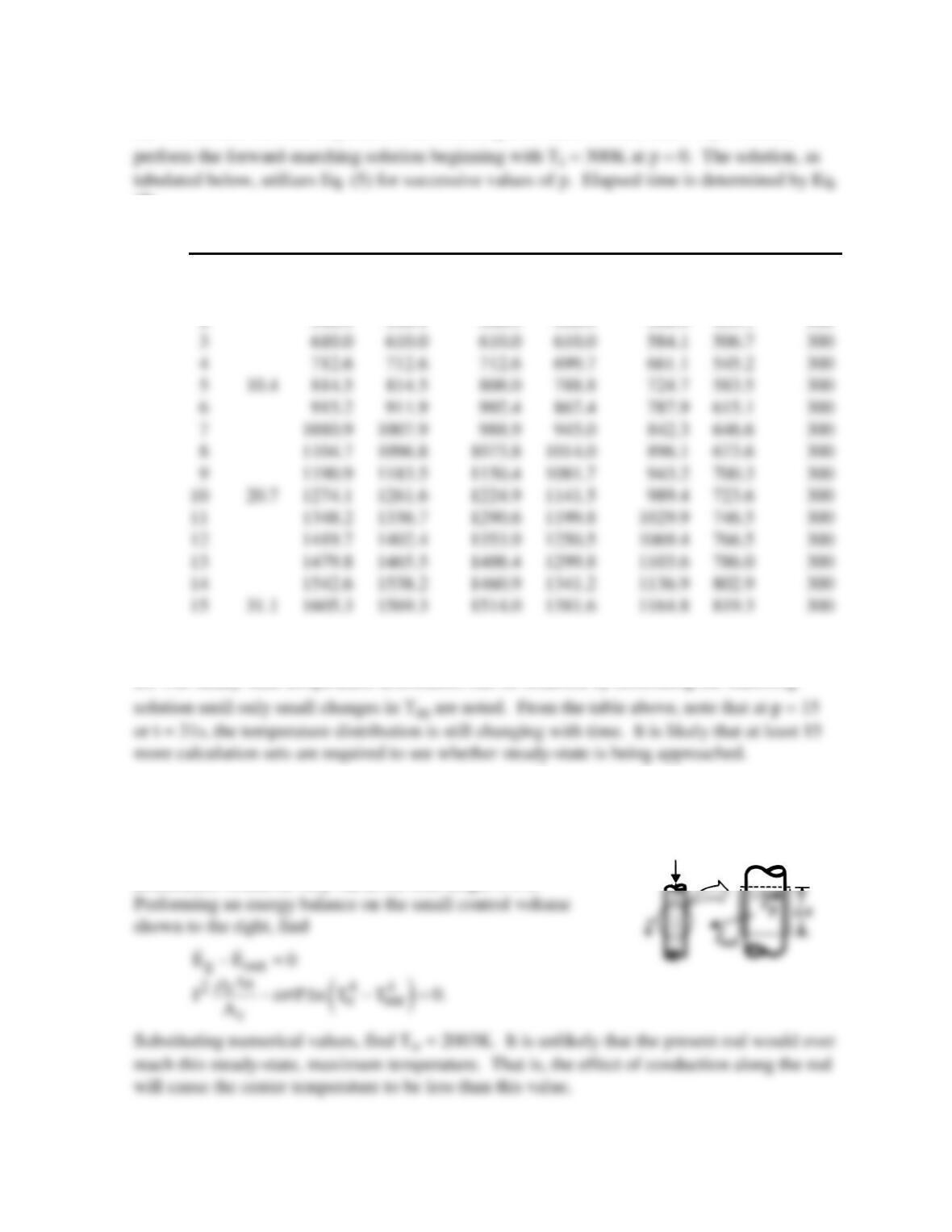
(a) To estimate the time required for the mid-length to reach 1000K, that is To = 1000K,
(7).
P t(s) T0 T1 T2 T3 T4 T5 T6(°C)
0 0 300 300 300 300 300 300 300
1 403.5 403.5 403.5 403.5 403.5 403.5 300
2 506.9 506.9 506.9 506.9 506.9 455.1 300
Note that, at p ≈ 6.9 or t = 6.9 × 2.07 = 14.3s, the mid-point temperature is To ≈ 1000K. <
(b) The steady-state temperature distribution can be obtained by continuing the marching
COMMENTS: (1) This problem should be solved with a computer rather than a hand-
calculator. For such a situation, it would be appropriate to decrease the spatial increment in
order to obtain better estimates of the temperature distribution.
(2) If the rod were very long, the steady–state temperature
distribution would be very flat at the mid-length x = 0.
PROBLEM 5.109
KNOWN: Support rod spanning a channel whose walls are maintained at Tb = 300 K. Suddenly the rod
is exposed to cross flow of hot gases with
T∞
= 600 K and h = 75 W/m2⋅K. After the rod reaches
steady–state conditions, the hot gas flow is terminated and the rod cools by free convection and radiation
exchange with surroundings.
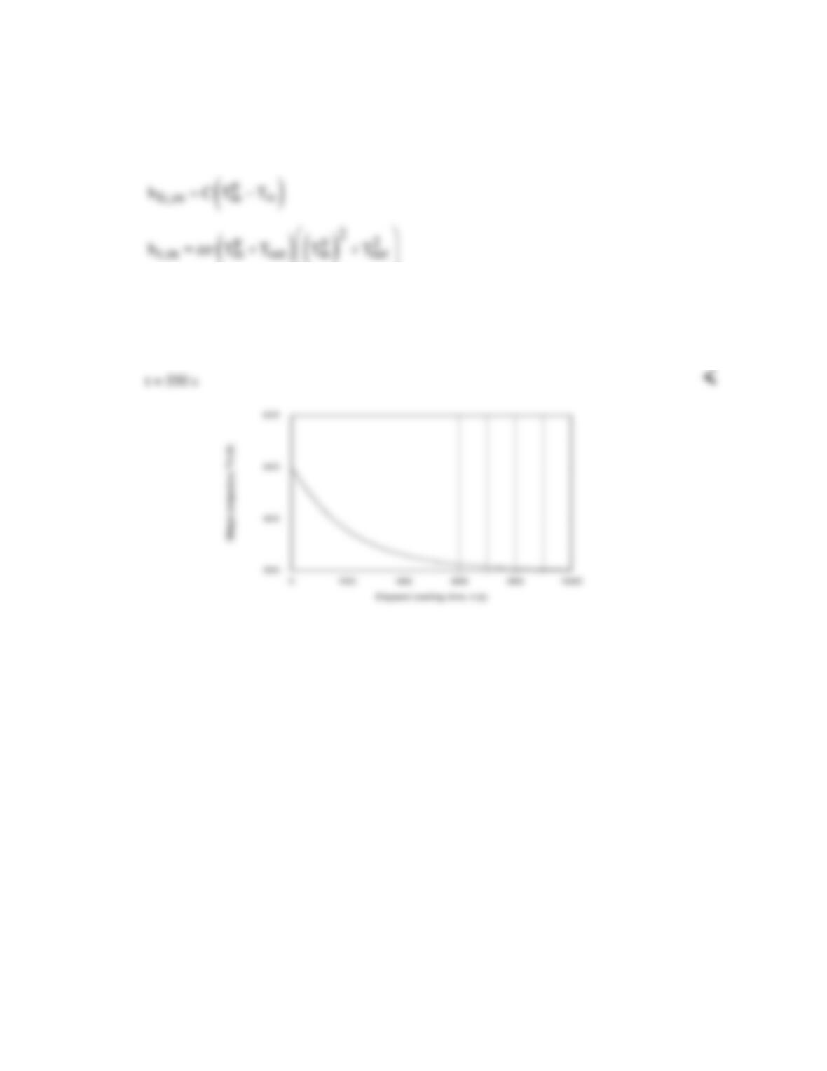
FIND: (a) Compute and plot the midspan temperature as a function of elapsed heating time; compare the
steady–state temperature distribution with results from an analytical model of the rod and (b) Compute
the midspan temperature as a function of elapsed cooling time and determine the time required for the
rod to reach the safe–to-touch temperature of 315 K.
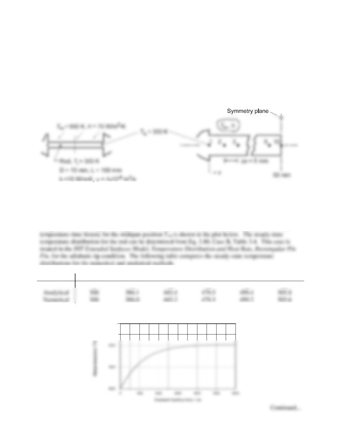
SCHEMATIC:
ASSUMPTIONS: (1) One-dimensional, transient conduction in rod, (2) Constant properties, (3) During
heating process, uniform convection coefficient over rod, (4) During cooling process, free convection
coefficient is of the form h = C∆Tn where C = 4.4 W/m2⋅K1.188 and n = 0.188, and (5) During cooling
process, surroundings are large with respect to the rod.
ANALYSIS: (a) The finite–difference equations for the 10-node mesh shown above can be obtained
using the IHT Finite-Difference Equation, One-Dimensional, Transient Extended Surfaces Tool. The
Method
Temperatures (K) vs. Position x (mm)
0
10
20
30
40
50
The comparison is excellent indicating that the nodal mesh is sufficiently fine to obtain precise results.
600
PROBLEM 5.109 (Cont.)
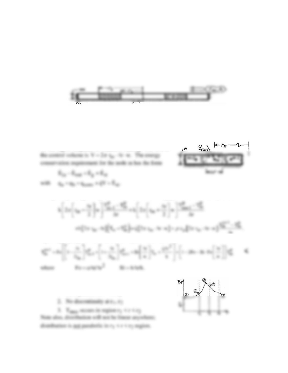
(b) The same finite–difference approach can be used to model the cooling process. In using the IHT tool,
the following procedure was used: (1) Set up the FDEs with the convection coefficient expressed as hm =
hfc,m + hr,m, the sum of the free convection and linearized radiation coefficients based upon nodal
temperature Tm.
(2) For the initial solve, set hfc,m = hr,m = 5 W/m2⋅K and solve, (3) Using the solved results as the Initial
Guesses for the next solve, allow hfc,m and hr,m to be unknowns. The temperature-time history for the
midspan during the cooling process is shown in the plot below. The time to reach the safe-to–touch
temperature,
T K
p
10 315=
, is
PROBLEM 5.110
KNOWN: Thin, circular-disc subjected to induction heating causing a uniform heat
generation in a prescribed region; upper surface exposed to convection process.
FIND: (a) Transient finite-difference equation for a node in the region subjected to induction
heating, (b) Sketch the steady–state temperature distribution on T-r coordinates; identify
important features.
SCHEMATIC:
ASSUMPTIONS: (1) Thickness w << ro, such that conduction is one-dimensional in r-
direction, (2) In prescribed region,
q
is uniform, (3) Bottom surface of disc is insulated, (4)
Constant properties.
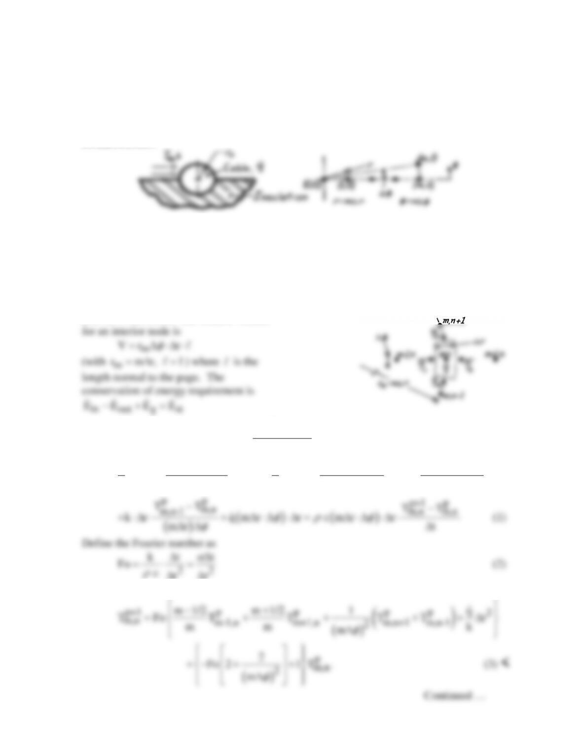
ANALYSIS: (a) Consider the nodal point arrangement
for the region subjected to induction heating. The size of
Recognizing that qa and qb are conduction terms and qconv is the convection process,
t
Upon regrouping, the finite-difference equation has the form,
(b) The steady–state temperature distribution has
these features:
1. Zero gradient at r = 0, r0
PROBLEM 5.111
KNOWN: An electrical cable experiencing uniform volumetric generation; the lower half is well
insulated while the upper half experiences convection.
FIND: (a) Explicit, finite-difference equations for an interior node (m,n), the center node (0,0), and
an outer surface node (M,n) for the convective and insulated boundaries, and (b) Stability criterion for
each FDE; identify the most restrictive criterion.
SCHEMATIC:
ASSUMPTIONS: (1) Two-dimensional (r,φ), transient conduction, (2) Constant properties, (3)
Uniform
q.
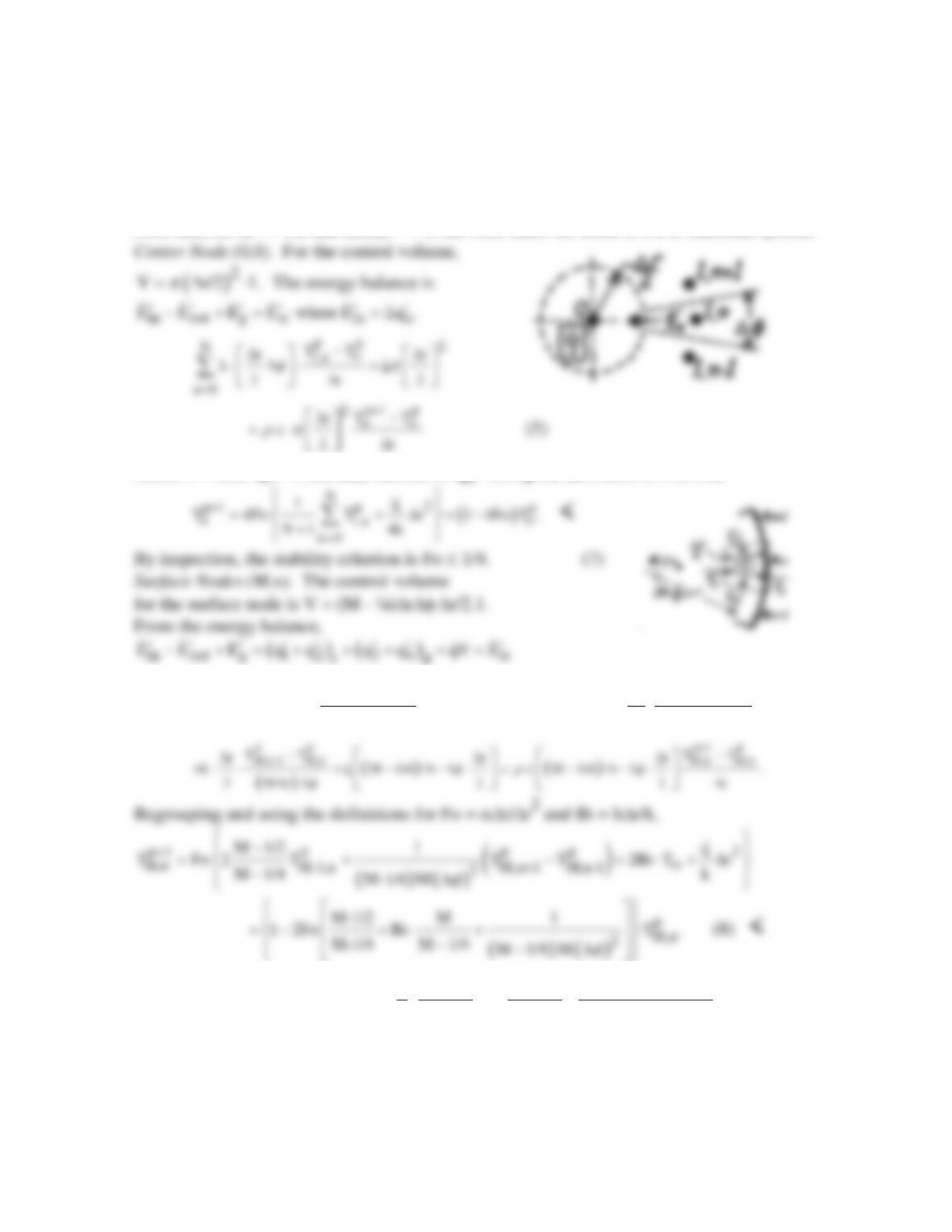
ANALYSIS: The explicit, finite–difference equations may be obtained by applying energy balances
to appropriate control volumes about the node of interest. Note the coordinate system defined above
where (r,φ) → (m∆r, n∆φ). The stability criterion is determined from the coefficient associated with
the node of interest.
Interior Node (m,n). The control volume
( ) ( )
p+1 p
m,n m,n
12 34
r
TT
q q q q qV cV t
θ
ρ
−
+ ++ += ∆
( )
p pp
p pp
m,n m,n m,n
m-1,n m+1,n m,n+1
TT T T TT
11
km r km r k r
2 r 2 r mr
φφ φ
− −−
⋅ − ∆ ⋅∆ ⋅ + ⋅ + ∆ ⋅∆ ⋅ + ⋅∆ ⋅
∆ ∆ ∆∆
∆∆
and then regroup the terms of Eq. (1) to obtain the FDE,
PROBLEM 5.111 (Cont.)
The stability criterion requires that the last term on the right-hand side in braces be positive. That is,
the coefficient of
p
m,n
T
must be positive and the stability criterion is
( )
2
Fo 1/2 1 1/ m
φ
≤ +∆
(4)
Note that, for m >> 1/2 and (m∆φ)2 >>1, the FDE takes the form of a 1–D cartesian system.
where N = (2π/∆φ) – 1, the total number of qn. Using the definition of Fo, find
( ) ( )
( )
( )
pp p p
M,n M,n
M-1,n M,n+1
p
M,n
TT TT
r
k M 1/2 r h M r T T +k
r 2 Mr
φφ φ
∞
−−
∆
⋅ − ∆ ⋅∆ + ∆ ⋅∆ − ⋅ ⋅
∆ ∆∆
The stability criterion is
( ) ( )
2
1 M 1/2 M 1
Fo Bi .
2 M 1/4 M 1/4 M 1/4 M
φ
−
≤ ++
−−
−∆
(9)
To determine which stability criterion is most restrictive, compare Eqs. (4), (7) and (9). The most
restrictive (lowest Fo) has the largest denominator. For small values of m, it is not evident whether
Eq. (7) is more restrictive than Eq. (4); Eq. (4) depends upon magnitude of ∆φ. Likewise, it is not
clear whether Eq. (9) will be more or less restrictive than Eq. (7). Numerical values must be
substituted.
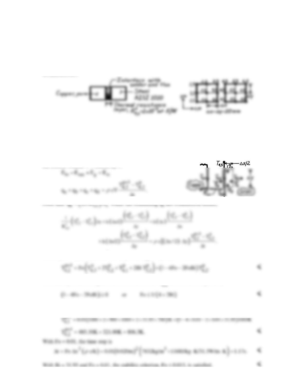
PROBLEM 5.112
KNOWN: Initial temperature distribution in two bars that are to be soldered together; interface
contact resistance.
FIND: (a) Explicit FDE
for T4,2
in terms of Fo and
t,c
Bi x/k R ;
′′
= ∆
stability criterion, (b) T4,2
one time step after contact is made if Fo = 0.01 and value of ∆t; whether the stability criterion is
satisfied.
SCHEMATIC:
PROPERTIES: Table A-1, Steel, AISI 1010 (1000K): k = 31.3 W/m⋅K, c = 1168 J/kg⋅K, ρ = 7832
kh/m3.
ASSUMPTIONS: (1) Two-dimensional transient conduction, (2) Constant properties, (3) Interfacial
solder layer has negligible thickness.
ANALYSIS: (a) From an energy balance on
the control volume V = (∆x/2)⋅∆y⋅1.
′′
Defining
( )
2c t,c
Fo k/ c t/ x and Bi y/R k,
ρ
′′
≡ ∆ ∆ ≡∆
regroup to obtain
The stability criterion requires the coefficient of the
p
T
term be zero or positive,
(b) For
()
-5 2
Fo 0.01 and Bi 0.020m/ 2 10 m K/W 31.3W/m K 31.95,= = × ⋅ × ⋅=
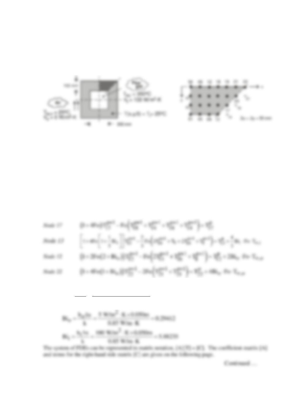
PROBLEM 5.113
KNOWN: Flue of square cross–section, initially at a uniform temperature, is suddenly exposed to hot
flue gases.
FIND: Temperature distribution in the wall and heat loss rate at 5, 10, 50 and 100 hours after
introduction of gases using the implicit finite-difference method.
SCHEMATIC:
ASSUMPTIONS: (1) Two-dimensional transient conduction, (2) Constant properties.
PROPERTIES: Flue (given): k = 0.85 W/m⋅K, α = 5.5 × 10⁻⁷ m2/s.
ANALYSIS: The network representing the flue cross–sectional area is shown with ∆x = ∆y = 50 mm.
Initially all nodes are at Ti = 25°C when suddenly the interior and exterior surfaces are exposed to
convection processes, (T∞,i, hi) and (T∞,o, ho), respectively Referring to the network above, note
that there are four types of nodes: interior (02, 03, 06, 07, 10, 11, 14, 15, 17, 18, 20); plane surfaces
with convection (interior – 01, 05, 09); interior corner with convection (13), plane surfaces with
convection (exterior – 04, 08, 12, 16, 19, 21); and, exterior corner with convection. The system of
finite–difference equations representing the network is obtained using IHT|Tools|Finite–difference
equations|Two-dimensional|Transient. The IHT code is shown in Comment 2 and the results for t = 5,
10, 50 and 100 hour are tabulated below.
Numerical values for the relevant parameters are (using a time step of one hour):
( )
62
22
t 5.5 10 m / s 3600s
Fo 7.92000
x0.050m
α
−
∆× ×
= = =
∆
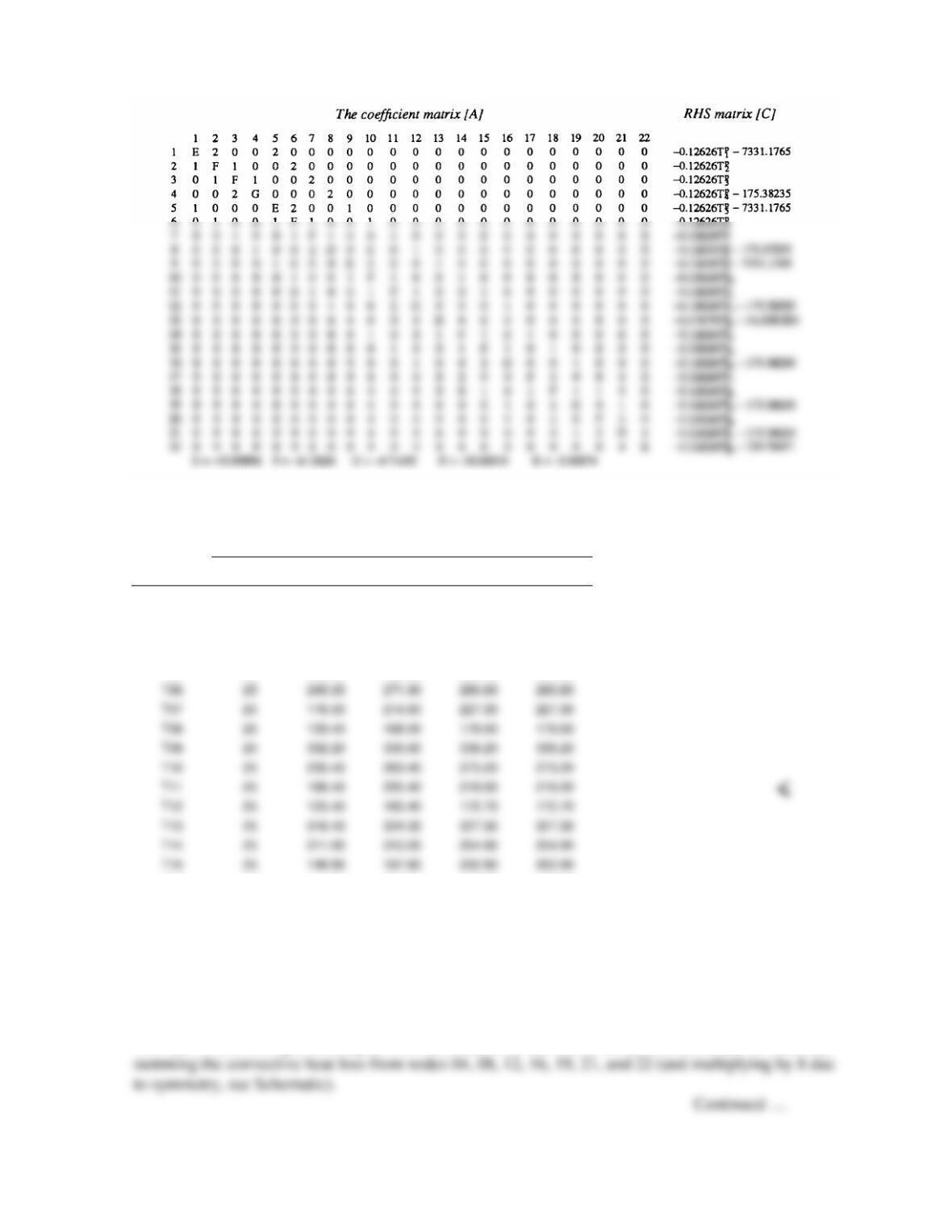
PROBLEM 5.113 (Cont.)
For this problem a standard computer program was used to obtain the solution matrix [T].
The initial temperature distribution was
0
m
T 25 C.= °
The results are tabulated below.
T(m,n) (C)
Node/time
(h)
0
5
10
50
100
T01
25
335.00
338.90
340.20
340.20
T02
25
248.00
274.30
282.90
282.90
T03
25
179.50
217.40
229.80
229.80
T04
25
135.80
170.30
181.60
181.60
T05
25
334.50
338.50
339.90
339.90
T16
25
110.90
146.70
160.20
160.20
T17
25
159.80
200.50
216.20
216.20
T18
25
117.40
160.50
177.50
177.50
T19
25
90.97
127.40
141.80
141.80
T20
25
90.62
132.20
149.00
149.00
T21
25
72.43
106.70
120.60
120.60
T22
25
59.47
87.37
98.89
98.89
The rate of heat loss (per unit depth) from the exterior of the flue to the environment can be found by
T06
25
245.30
271.90
280.80
280.80
T07
25
176.50
214.60
227.30
227.30
T08
25
133.40
168.00
179.50
179.50
T09
25
332.20
336.60
338.20
338.20
T10
25
235.40
263.40
273.20
273.20
T11
25
166.40
205.40
219.00
219.00
T12
25
125.40
160.40
172.70
172.70
T13
25
316.40
324.30
327.30
327.30
T14
25
211.00
243.00
254.90
254.90
T15
25
146.90
187.60
202.90
202.90
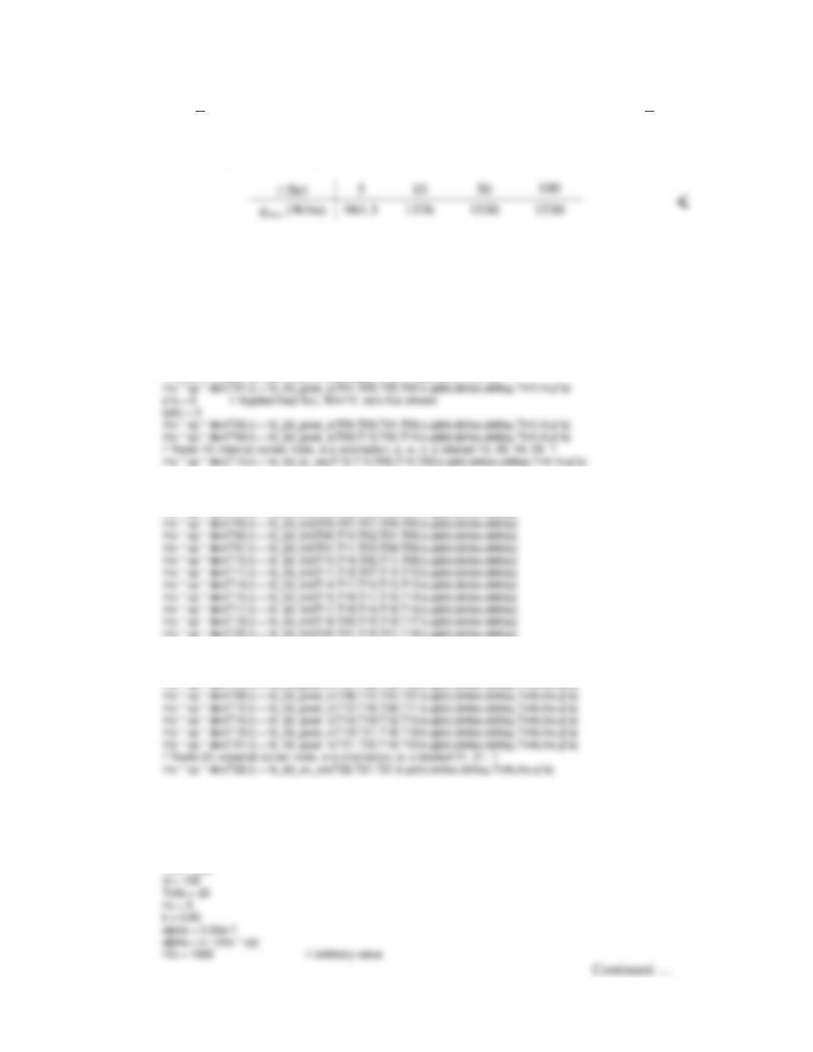
PROBLEM 5.113 (Cont.)
loss 4 , 8 , 12 , 16 , 19 , 21 , 22 ,
11
8 ( )( )( )( )( )( ) ( )
22
o oooooo o
qhxTTTTTTTTTTTT TT
∞∞∞∞∞∞ ∞
=∆ −+−+−+−+−+−+ −
The results for the different times are shown below.
COMMENTS: (1) Note that the steady–state condition is reached by t = 50 hours; this can be seen
by comparing the distributions for t = 50 and 100 hours. Within 10 hours, the flue is within a few
degrees of the steady–state condition and the heat loss rate is within 10% of the steady–state value. (2)
The IHT code for performing the numerical solution is shown in its entirety below. Use has been
made of symmetry in writing the FDEs. The tabulated results above were obtained by copying from
the IHT Browser and pasting the desired columns into EXCEL.
// From Tools|Finite–difference equations|Two-dimensional|Transient
// Interior surface nodes, 01, 05, 09, 13
/* Node 01: plane surface node, s–orientation; e, w, n labeled 05, 05, 02 . */
// Interior nodes, 02, 03, 06, 07, 10, 11, 14, 15, 18, 20
/* Node 02: interior node; e, w, n, s labeled 06, 06, 03, 01. */
rho * cp * der(T02,t) = fd_2d_int(T02,T06,T06,T03,T01,k,qdot,deltax,deltay)
rho * cp * der(T20,t) = fd_2d_int(T20,T21,T18,T21,T18,k,qdot,deltax,deltay)
// Exterior surface nodes, 04, 08, 12, 16, 19, 21, 22
/* Node 04: plane surface node, n–orientation; e, w, s labeled 08, 08, 03. */
// Rate of heat loss from nodes 04, 08, 12, 16, 19, 21, 22
qloss = 8*ho*deltax*((0.5*T04+T08+T12+T16+T19+T21+0.5*T22)–6*Tinfo)
// Input variables
deltax = 0.050
deltay = 0.050
Tinfi = 350

PROBLEM 5.113 (Cont.)
(3) The results for t = 50 hour, representing the steady-state condition, are shown below, arranged
according to the coordinate system.
Tmn (C)
x/y (mm)
0
50
100
150
200
250
300
0
181.60
179.50
172.70
160.20
141.80
120.60
98.89
Compared to the steady–state temperature distribution determined using a finer mesh (not shown), ∆x
= ∆y = 25 mm, the results for the coarser mesh are slightly higher, within a fraction of 1°C, along the
50
229.80
227.30
219.00
202.90
177.50
149.00
100
282.90
280.80
273.20
172.70
216.20
150
340.20
339.90
338.20
327.30
PROBLEM 5.114
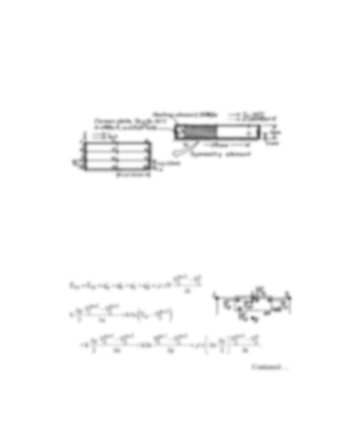
KNOWN: Electrical heating elements embedded in a ceramic plate of known properties and
dimensions. Environmental temperature and heat transfer coefficient. Initially plate is at a
uniform temperature and suddenly heaters are energized with known heat rate.
FIND: Time required for the difference between the surface above a heating element and
initial temperatures to reach 95% of the difference for steady–state conditions using the
implicit finite–difference method.
SCHEMATIC:
ASSUMPTIONS: (1) Two-dimensional conduction, (2) Constant properties, (3) No internal
generation except for Node 7, (4) Heating element approximates a line source; wire diameter
is negligible.
ANALYSIS: The grid for the symmetry element above consists of 12 nodes. Nodes 1-3 are
points on a surface experiencing convection; nodes 4-12 are interior nodes; node 7 is a special
case with internal generation and because of symmetry,
ht
q 25 W/m.
′=
Their finite–
difference equations are derived as follows.
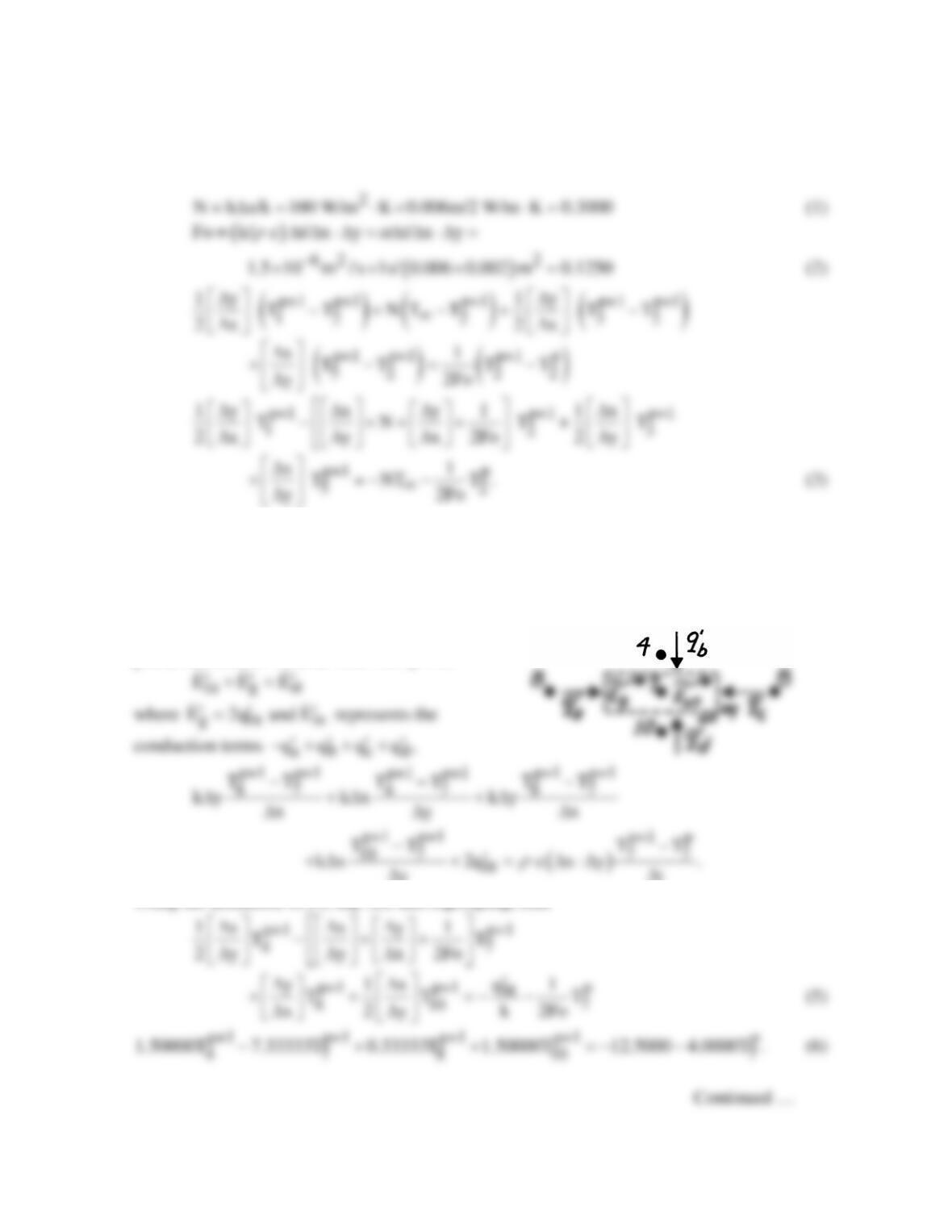
Surface Node 2. From an energy balance on the prescribed control volume with ∆x/∆y = 3,
PROBLEM 5.114 (Cont.)
Divide by k, use the following definitions, and regroup to obtain the finite-difference
equations.
Substituting numerical values for Fo and N, and using T∞ = 30°C and ∆x/∆y = 3, find
p+1 p+1 p+1 p+1 p
5
123 2
0.16667T 7.63333T 0.16667T 3.00000T 9.0000 4.0000T .−++=−
(4)
By inspection and use of Eq. (3), the FDEs for Nodes 1 and 3 can be inferred.
Interior Node 7. From an energy balance on the
prescribed control volume with ∆x/∆y = 3,
yt
∆∆
Using the definition of Fo, Eq. (2), and regrouping, find
PROBLEM 5.114 (Cont.)
Recognizing the form of Eq. (5), it is a simple matter to infer the FDE for the remaining
interior points for which
ht
q 0.=
In matrix notation [A][T] = [C], the coefficient matrix [A]
and RHS matrix [C] are:
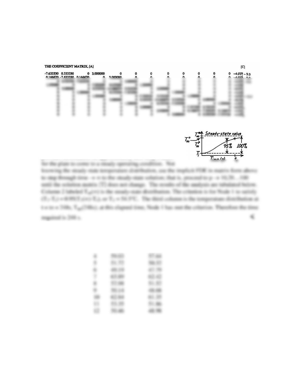
Recall that the problem asks for the time required for the
surface temperature difference (relative to the initial
temperature) above a heating element (Node 1) to reach
95% of the difference for steady-state conditions. This
provides information on approximately how long it takes
m Tm(∞) Tm(248s)
1 55.80 54.51
2 49.93 48.64
3 47.67 46.38
COMMENTS: Note that at t = 248 s, the only nodes that have met the 95% criterion are
Nodes 1, 4, 7, and 10. Can you explain these nodes were the first to reach this limit? Which
nodes will be the last to reach their limits?
PROBLEM 5S.1
KNOWN: Configuration, initial temperature and charging conditions of a thermal energy storage
unit.
FIND: Time required to achieve 75% of maximum possible energy storage and corresponding
minimum and maximum temperatures.
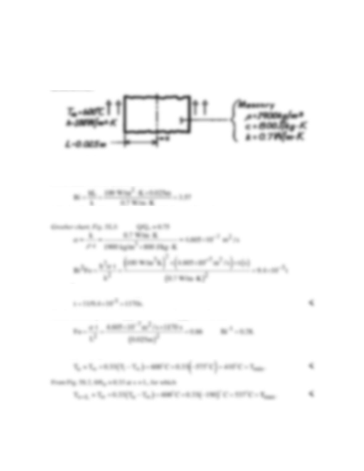
SCHEMATIC:
ASSUMPTIONS: (1) One-dimensional conduction, (2) Constant properties, (3) Negligible radiation
exchange with surroundings.
ANALYSIS: For the system, find first
indicating that the lumped capacitance method cannot be used.
Find Bi2Fo ≈ 11, and substituting numerical values
Heisler chart, Fig. 5S.1: Tmin is at x = 0 and Tmax at x = L, with
From Fig. 5S.1,
o
0.33.
θ
∗
≈
Hence,
COMMENTS: If the storage unit were made of aluminum (Al), rather than masonry (m), (ρc)Al >
(ρc)m and kAl > km. Hence, the aluminum can store more energy and can be charged (or
discharged) more quickly.
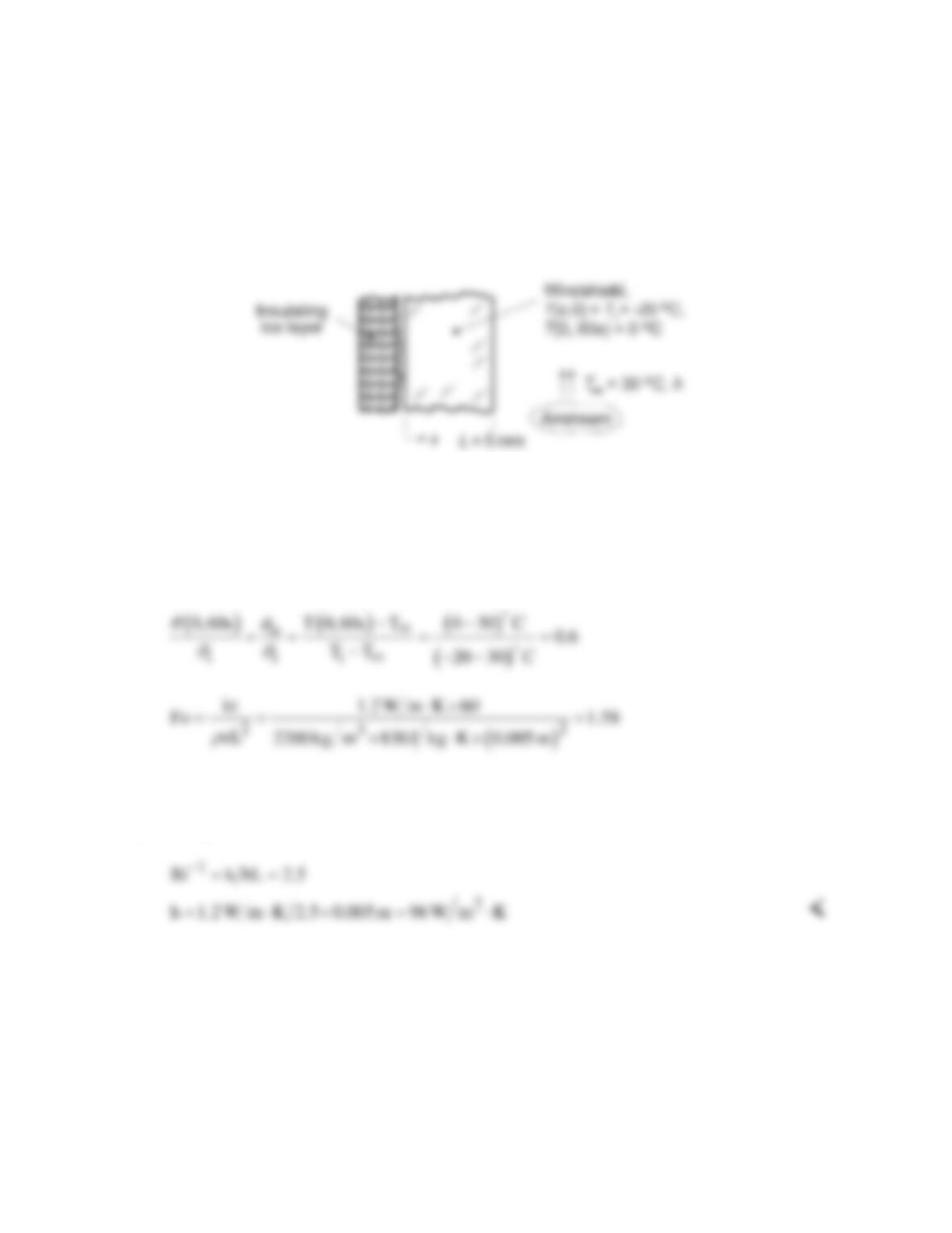
PROBLEM 5S.2
KNOWN: Car windshield, initially at a uniform temperature of –20°C, is suddenly exposed on its
interior surface to the defrost system airstream at 30°C. The ice layer on the exterior surface acts as an
insulating layer.
FIND: What airstream convection coefficient would allow the exterior surface to reach 0°C in 60 s?
SCHEMATIC:
ASSUMPTIONS: (1) One-dimensional, transient conduction in the windshield, (2) Constant properties,
(3) Exterior surface is perfectly insulated.
PROPERTIES: Windshield (Given): ρ = 2200 kg/m3, cp = 830 J/kg⋅K and k = 1.2 W/m⋅K.
ANALYSIS: For the prescribed conditions, from Equations 5.34 and 5.36,
The single-term series approximation, Eq. 5.44, along with Table 5.1, requires an iterative solution to
find an appropriate Biot number. Alternatively, the Heisler charts, Section 5S.1, Figure 5S.1, for the
midplane temperature could be used to find
COMMENTS: Using the IHT, Transient Conduction, Plane Wall Model, the convection coefficient
can be determined by solving the model with an assumed h and then sweeping over a range of h until the
T(0,60s) condition is satisfied. Since the model is based upon multiple terms of the series, the result of h
= 99 W/m2⋅K is more precise than that found using the chart.