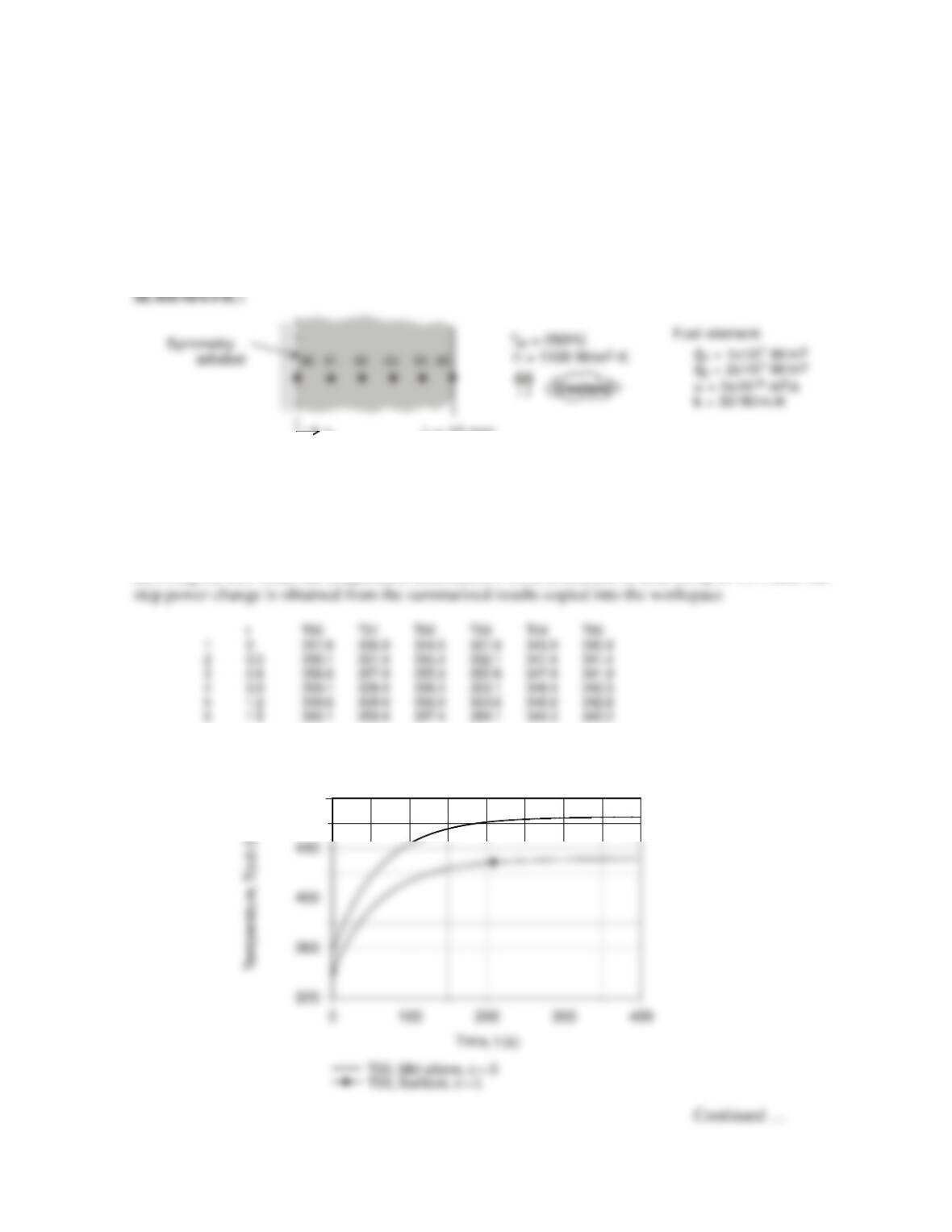
Chapter 5 Hot dog with prescribed thermophysical properties

PROBLEM 5.100

KNOWN: Conditions associated with heat generation in a rectangular fuel element with surface

cooling. See Example 5.11.

FIND: (a) The temperature distribution 1.5 s after the change in operating power; compare your

results with those tabulated in the example, (b) Calculate and plot temperature histories at the mid–

plane (00) and surface (05) nodes for 0≤ t ≤ 400 s; determine the new steady–state temperatures, and

approximately how long it will take to reach the new steady-state condition after the step change in

operating power. Use the IHT Tools | Finite-Difference Equations | One-Dimensional | Transient

conduction model builder as your solution tool.

L = 10 mm

x

ASSUMPTIONS: (1) One dimensional conduction in the x-direction, (2) Uniform generation, and (3)

Constant properties.

ANALYIS: The IHT model builder provides the transient finite-difference equations for the implicit

method of solution. Selected portions of the IHT code used to obtain the results tabulated below are

shown in the Comments.

(a) Using the IHT code, the temperature distribution (°C) as a function of time (s) up to 1.5 s after the

(b) Using the code, the mid-plane (00) and surface (05) node temperatures are plotted as a function of

time.

Temperature history after step change in power

480

PROBLEM 5.100 (Cont.)

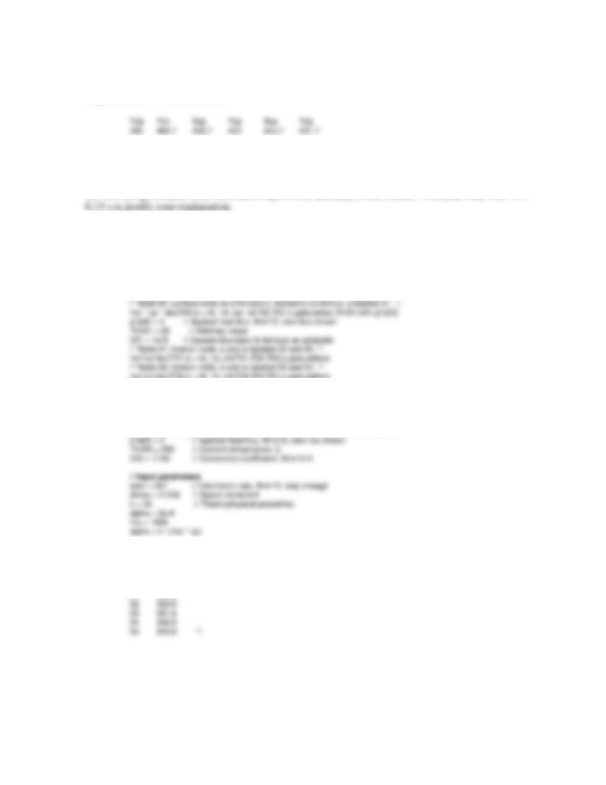
Note that at t ≈ 240 s, the wall has nearly reached the new steady–state condition for which the nodal

temperatures (°C) were found as:

COMMENTS: (1) Can you validate the new steady–state nodal temperatures from part (b) by

comparison against an analytical solution?

(2) Will using a smaller time increment improve the accuracy of the results? Use your code with ∆t =

(3) Selected portions of the IHT code to obtain the nodal temperature distribution using spatial and

time increments of ∆x = 2 mm and ∆t = 0.3 s, respectively, are shown below. For the solve-

integration step, the initial condition for each of the nodes corresponds to the steady-state temperature

distribution with

1

q.



// Tools | Finite–Difference Equations | One–Dimensional | Transient

rho*cp*der(T02,t) = fd_1d_int(T02,T03,T01,k,qdot,deltax)

/* Node 03: interior node; e and w labeled 04 and 02. */

rho*cp*der(T03,t) = fd_1d_int(T03,T04,T02,k,qdot,deltax)

/* Node 04: interior node; e and w labeled 05 and 03. */

rho*cp*der(T04,t) = fd_1d_int(T04,T05,T03,k,qdot,deltax)

/* Node 05: surface node (e–orientation); transient conditions; w labeled 04. */

rho * cp * der(T05,t) = fd_1d_sur_e(T05,T04,k,qdot,deltax,Tinf05,h05,q”a05)

/* Steady–state conditions, with qdot1 = 1e7 W/m^3; initial conditions for step change

T_x = 16.67 * (1 – x^2/L^2) + 340.91 // See text

Seek T_x for x = 0, 2, 4, 6, 8, 10 mm; results used for Ti are

Node T_x

00 357.6

01 356.9

PROBLEM 5.101

KNOWN: Thickness and thermal diffusivity of a plane wall. Initial and boundary conditions.

FIND: (a) Temperature distribution at t = 30 min using an explicit finite difference technique with a

time step of 600 s and a space increment of 30 mm. (b) Temperature distribution at t = 30 min using

an implicit finite difference technique with a time step of 600 s and a space increment of 30 mm.

ASSUMPTIONS: (1) One-dimensional heat transfer, (2) Constant properties.

PROPERTIES: Thermal diffusivity,



= 1.5  10-6 m2/s (given).

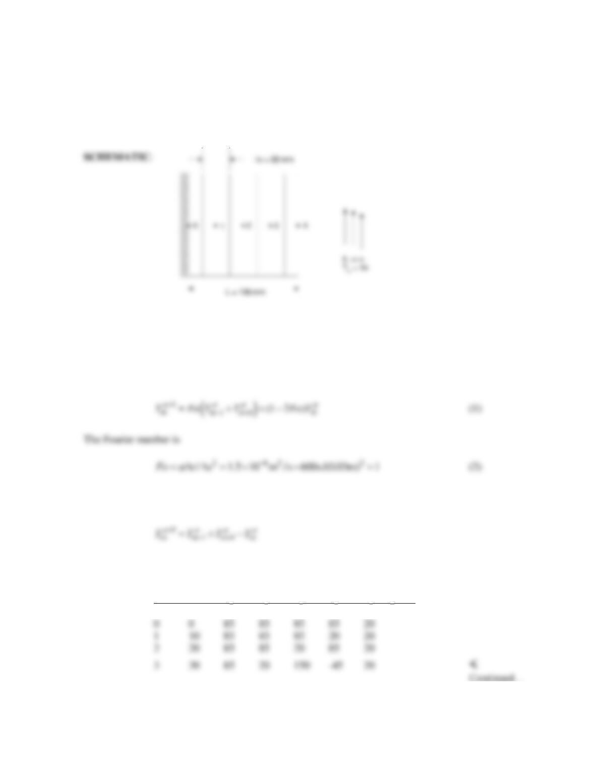
ANALYSIS: (a) The finite-difference equations for the interior points, nodes 0, 1, 2 and 3, can be

determined from Eq. 5.81,

Note that the stability criterion of Eq. 5.82 is not satisfied. Nonetheless, we will combine Eqs. (1) and

(2) to yield

Since the adiabatic surface at x = 0 can be treated as a symmetry plane, we note that Tm-1 = Tm+1 for

node 0. The finite-difference solution is shown in the table below.

p t (min) T0 T1 T2 T3 T4 = TL (C)

PROBLEM 5.101 (Cont.)

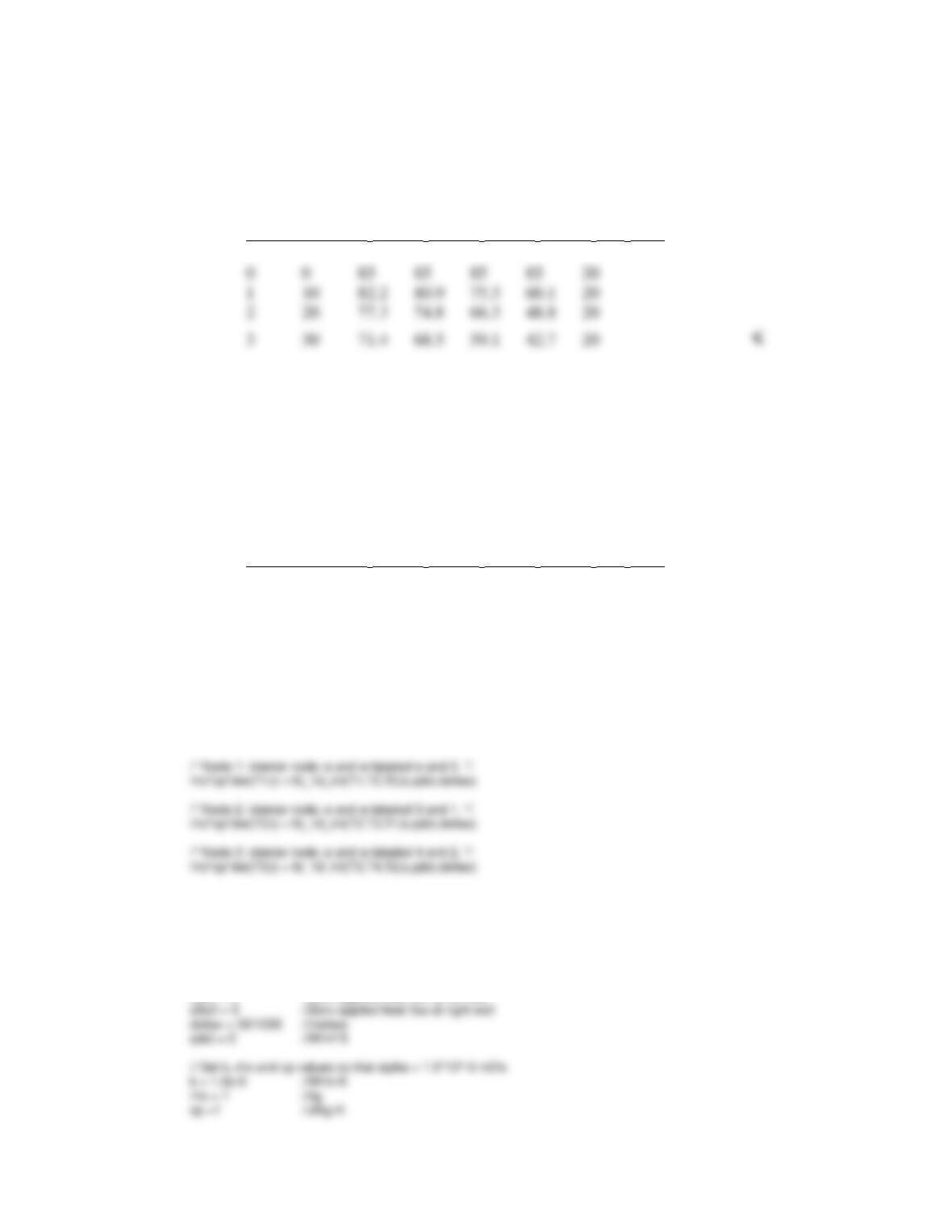
(b) Note that for this solution, the conditions at the right face have been incorporated by specifying a

very large convection coefficient at the right face so that T4  T. The IHT code is shown in the

COMMENTS section. The following results were obtained.

p t (min) T0 T1 T2 T3 T4 = TL (C)

COMMENTS: (1) The IHT Code for part (b) is shown at the end of the Comments. (2) Note the

thermal response of part (a) is unrealistic. This unrealistic result is expected since the stability criterion

is not satisfied. (3) Part (b) was repeated with a smaller time step of t = 300 s yielding the following

results. Note that these results differ from those associated with the larger time step. Just because the

implicit finite-difference method is inherently stable, the solutions may still be dependent upon the

time step and, as such, are incorrect.

p t (min) T0 T1 T2 T3 T4 = TL (C)

0 0 85 85 85 85 20

1 10 82.8 81.2 74.8 57.5 20

2 20 77.7 74.8 65.3 46.9 20

3 30 71.3 68.1 58.1 41.4 20

/* Node 0: surface node (w-orientation); transient conditions; e labeled 1. */

rho * cp * der(T0,t) = fd_1d_sur_w(T0,T1,k,qdot,deltax,Tinf,h1,qfla0)

/* Node 4: surface node (e-orientation); transient conditions; w labeled 3. */

rho * cp * der(T4,t) = fd_1d_sur_e(T4,T3,k,qdot,deltax,Tinf,h2,qfla4)

Tinf = 20 //Initial Conditions are T = 85 everywhere (C)

h1 = 0 //Insulated left wall

h2 = 1e10 //Right wall at Tinf since h2 is nearly infinite

qfla0 = 0 //Zero applied heat flux at left wall

PROBLEM 5.102

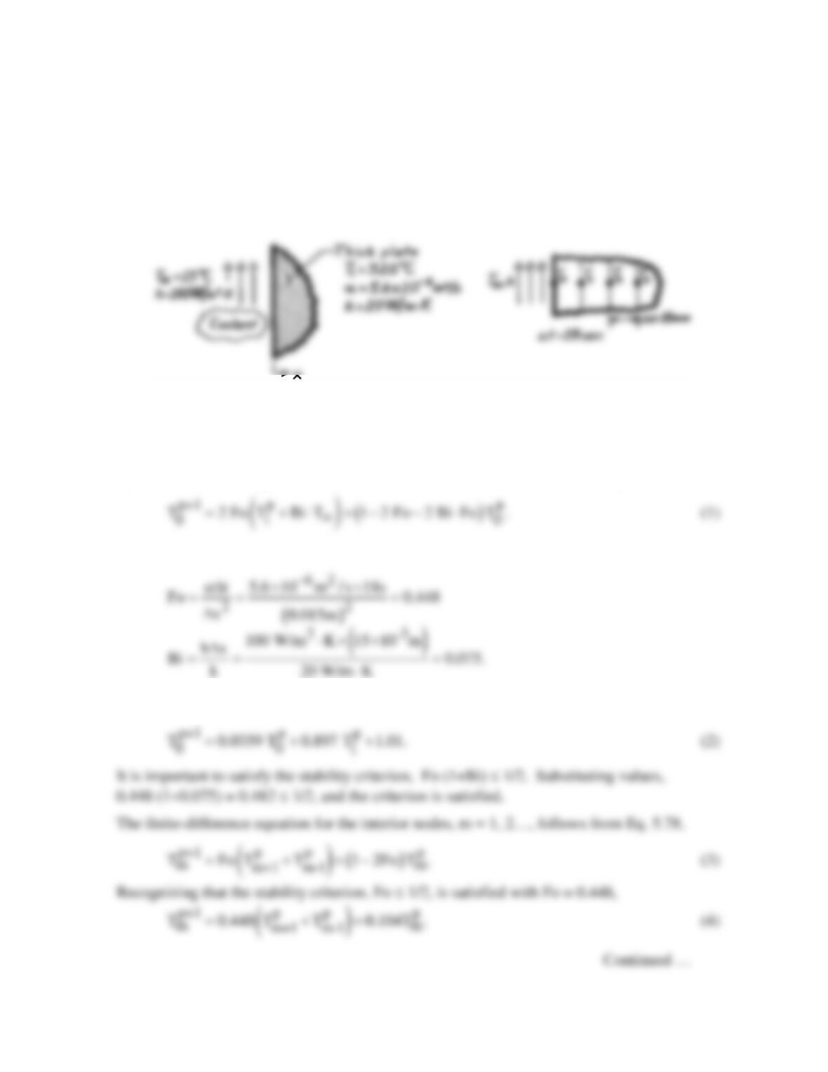
KNOWN: Very thick plate, initially at a uniform temperature, Ti, is suddenly exposed to a

convection cooling process (T∞,h).

FIND: Temperatures at the surface and a 45mm depth after 3 minutes using finite-difference

method with space and time increments of 15mm and 18s.

SCHEMATIC:

ASSUMPTIONS: (1) One-dimensional transient conduction, (2) Plate approximates semi-

infinite medium, (3) Constant properties.

ANALYSIS: The grid network representing the plate is shown above. The finite-difference

equation for node 0 is given by Eq. 5.90 for one-dimensional conditions or Eq. 5.85,

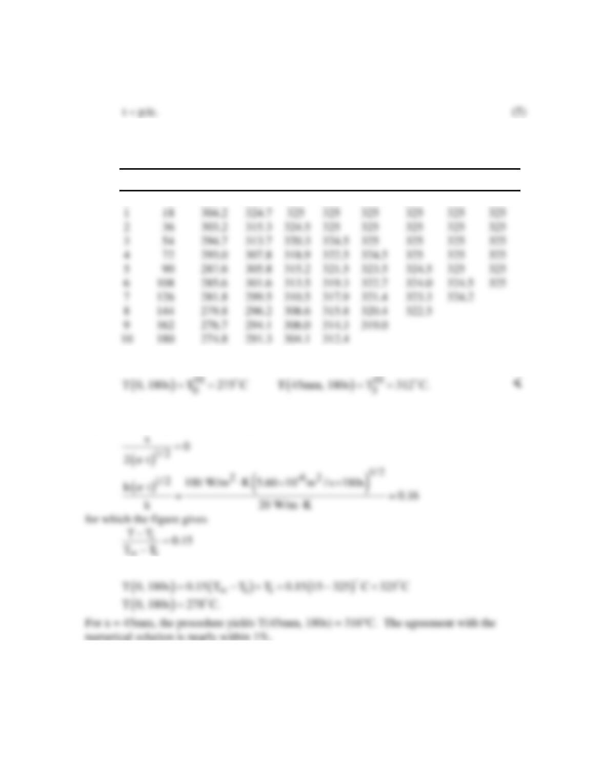
The numerical values of Fo and Bi are

Recognizing that T∞ = 15°C, Eq. (1) has the form

PROBLEM 5.102 (Cont.)

The time scale is related to p, the number of steps in the calculation procedure, and ∆t, the

time increment,

The finite-difference calculations can now be performed using Eqs. (2) and (4). The results

are tabulated below.

p t(s) T0 T1 T2 T3 T4 T5 T6 T7(K)

0 0 325 325 325 325 325 325 325 325

Hence, find

COMMENTS: (1) The above results can be readily checked against the analytical solution

represented in Fig. 5.8 (see also Eq. 5.63). For x = 0 and t = 180s, find

i

∞

so that,

PROBLEM 5.103

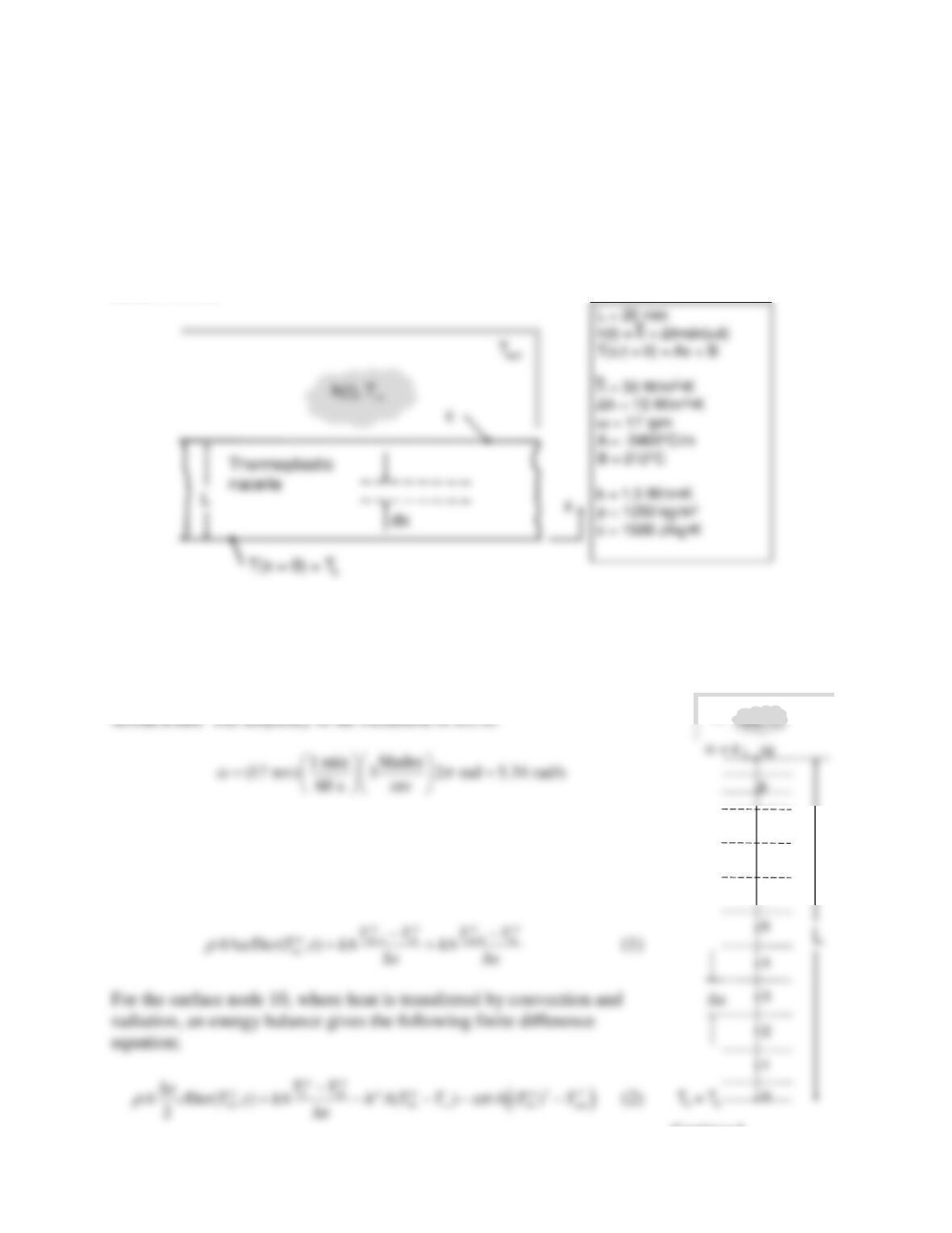
KNOWN: Thickness and thermophysical properties of wind turbine nacelle of Example 3.1. Rotational

speed and number of blades. Average value and amplitude of sinusoidal variation of heat transfer

coefficient versus time. Initial wall temperature distribution.

FIND: Transient wall temperature distribution for

40 50 s,t≤≤

using ∆x = 2 mm and ∆t = 0.05 s. Plot of

exterior nacelle surface temperature, exterior surface convection heat flux, and exterior surface radiation

heat flux for

40 50 s.t≤≤

Explain.

SCHEMATIC:

ASSUMPTIONS: (1) One-dimensional plane wall, (2) Uniform properties, (3) Large surroundings,

α

=

ε

, (4) Ts = constant.

PROPERTIES: Given,

ρ

= 1250 kg/m3, c = 1500 J/kg⋅K, k = 1.5 W/m⋅K.

The nodal layout is shown in the schematic to the right. The finite difference

equation for internal nodes 1 through 9 is the same as in Example 5.11 (with

q



= 0), except that we write the time derivative in terms of the Der function of

IHT:

Continued…

7

6

8

Tsur

PROBLEM 5.103 (Cont.)

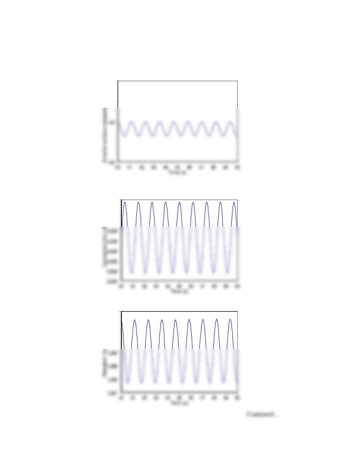
Equations (1) and (2) are implemented in the IHT code shown in the Comments section. The

solution for the nacelle temperature, convection heat flux, and radiation heat flux at the exterior

surface are plotted below.

144

6,000

5,500

5,000

1,063

1,062

1,061

PROBLEM 5.103 (Cont.)

The initial predicted response (t ≅ 0) is not shown. The behavior for

40 50 st≤≤

corresponds to quasi-

steady behavior. The time-varying convection heat transfer coefficient leads to time variation of the

exterior surface temperature, which in turn leads to time varying exterior heat fluxes and time variation of

temperatures internal to the wall.

COMMENTS: (1) The IHT code is shown below.

// T10 at exposed surface, T0 at inner surface

//Properties,dimensions

k = 1.5

dx = 0.002

//Convective conditions outside nacelle

h = hbar + delh*sin(omega*t)

//17 rpm rotors, 3 blades

omega = 17*3*2*pi/60

//Radiative conditions

eps = 0.83

sigma = 5.67e-8

Tsur = 20 + 273

//Node 0

T0 = 212

//Nodes 1 through 9

Ac = 1

rhoc*dx*Ac*Der(T1,t) = Ac*k/dx*(T0 – T1) + Ac*k/dx*(T2 – T1)

qradflux =eps*sigma*Ac*((T10 + 273)^4 – Tsur^4)

qconflux = h*Ac*(T10 – Tinf)

Continued…

PROBLEM 5.103 (Cont.)

//Initial conditions. Enter into IHT initial condition window.

//T0i = 212

//T1i = T0i – 3460*dx = 205.1

//T2i = T1i – 3460*dx = 198.2

(2) The time-averaged exterior total heat flux is 5187 W/m2. (3) The magnitudes of the various fluctuating

quantities depend on the thermophysical properties of the nacelle. Try some parametric simulations!

PROBLEM 5.104

KNOWN: Sudden exposure of the surface of a thick slab, initially at a uniform temperature,

to convection and to surroundings at a high temperature.

FIND: (a) Explicit, finite-difference equation for the surface node in terms of Fo, Bi, Bir, (b)

Stability criterion; whether it is more restrictive than that for an interior node and does it

change with time, and (c) Temperature at the surface and at 30mm depth for prescribed

conditions after 1 minute exposure.

SCHEMATIC:

ASSUMPTIONS: (1) One-dimensional transient conduction, (2) Thick slab may be

approximated as semi-infinite medium, (3) Constant properties, (4) Radiation exchange is

between small surface and large surroundings.

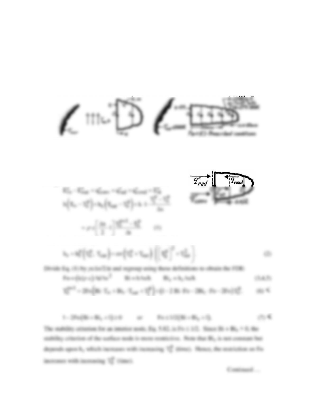
ANALYSIS: (a) The explicit form of the FDE for

the surface node may be obtained by applying an

energy balance to a control volume about the node.

where the radiation process has been linearized, Eq. 1.9.

(b) The stability criterion for Eq. (6) requires that the coefficient of

p

o

T

be positive.

PROBLEM 5.104 (Cont.)

(c) Consider the prescribed conditions with negligible convection (Bi = 0). The FDEs for the

thick slab are:

To proceed with the explicit, marching solution, we need to select a value of ∆t (Fo) that will

satisfy the stability criterion. A few trial calculations are helpful. A value of ∆t = 15s

provides Fo = 0.105, and using Eqs. (2) and (5), hr(300K, 1000K) = 72.3 W/m2⋅K and Bir =

0.482. From the stability criterion, Eq. (10), find Fo ≤ 0.337. With increasing

p

o

T,

hr and Bir

p

o

p t(s)

T h Bi

o r

pr

/ /

T1(K) T2 T3 T4 ….

0 0 300 300 300 300 300

72.3

0.482

COMMENTS: (1) The form of the FDE representing the surface node agrees with Eq. 5.90

if this equation is reduced to one-dimension.

(2) We should recognize that the ∆t = 15s time increment represents a coarse step. To

improve the accuracy of the solution, a smaller ∆t should be chosen.

PROBLEM 5.105

KNOWN: One-dimensional convective heating and cooling of a plane slab with Bi1 = 10 (for Heating

Phase 1, beginning at Fo = 0 and ending at Fo = Fo1 = 0.1), Bi2 = 1 (for Cooling Phase 2, beginning at

Fo = Fo1).

FIND: (a) Dimensionless form of the heat equation, initial and boundary conditions for Phase 1, (b)

Dimensionless form of the heat equation, initial and boundary conditions for Phase 2, (c) Finite

difference solution for

*

0



(x* = 1, Fo),

*

0



(x* = 0, Fo) and

*

0



(x* = 0.5, Fo) for Fo1 = 0.1 over the

range 0  Fo  0.5 using x* = 0.1 and Fo = 0.001, (d) Value of and time associated with the

minimum dimensionless temperature at the midplane of the wall.

SCHEMATIC:

ASSUMPTIONS: (1) One-dimensional conduction, (2) Constant properties.

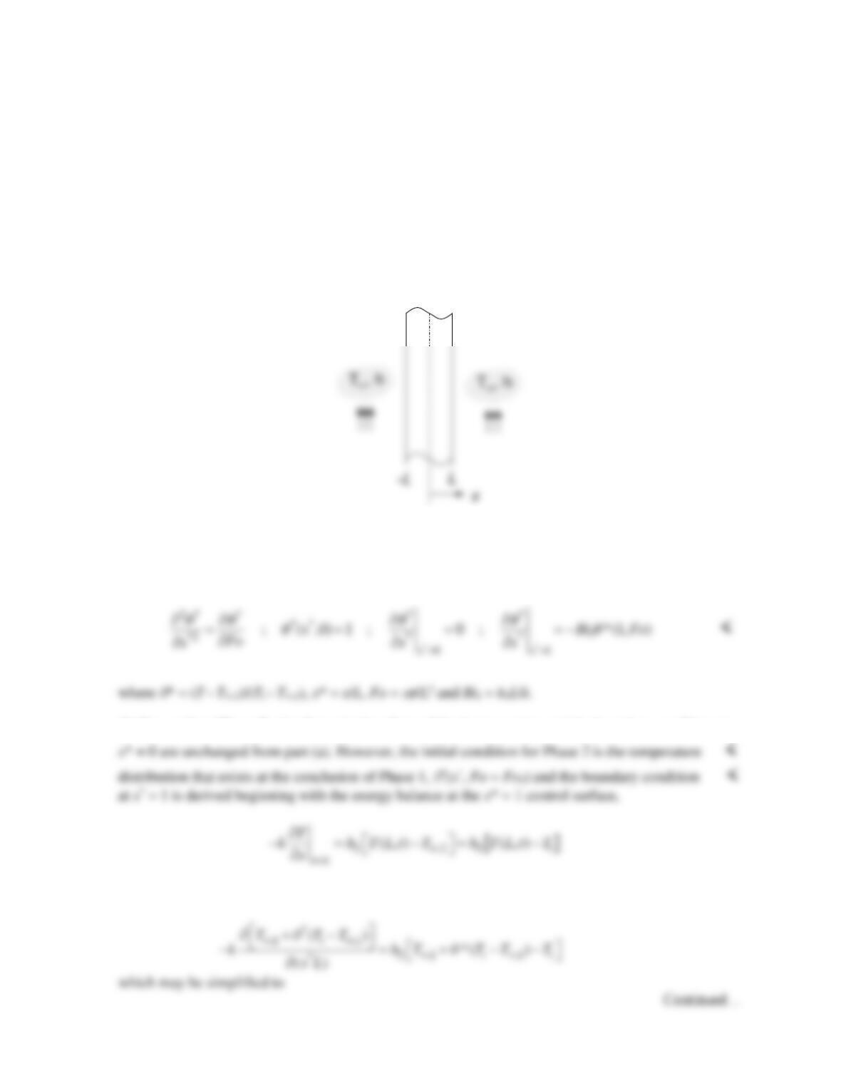
ANALYSIS: (a) The dimensionless forms of the heat equation, initial and boundary conditions for

Phase 1 are given by Eqs. 5.37 through 5.40,

(b) For cooling (Phase 2), the dimensionless form of the heat equation and the boundary condition at

Substituting the expressions T =



*(Ti – T,1) + T,1 and x = x*L into the preceding equation yields

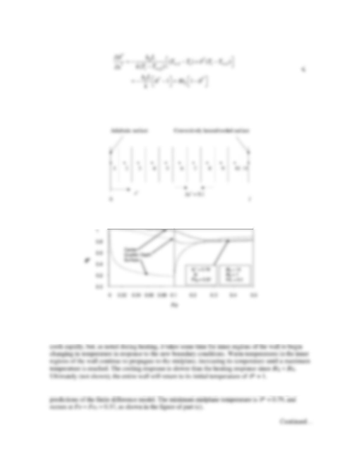
PROBLEM 5.105 (Cont.)

(c) The dimensionless form of the energy equation, based upon the discretization shown below, was

solved using IHT software. The IHT code is included in the comments.

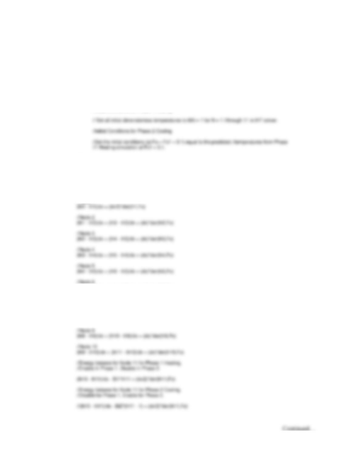
The thermal response is shown in the graph below.

Note that the surface heats quickly in Phase 1 (



* decreases rapidly) while the center midplane

temperature changes only slightly over the heating time. The quarter plane (or quarter depth)

temperature increases at an intermediate rate during heating. During cooling (Phase 2), the surface

(d) The minimum dimensionless temperature at the midplane may be determine by inspecting the

PROBLEM 5.105 (Cont.)

COMMENTS: (1) The IHT code used in part (c) is listed below.

// Boundary Conditions.

Bi1 = 10

Bi2 = 1

//Initial Conditions.

//Initial Conditions for Phase 1 Heating

//Control volume size.

dx = 0.1

//Node 1 is at the midplane.

//Node 11 is at the surface.

//Write energy balances for Nodes 1 through 10.

//Node 1

(th5 – th6)/dx + (th7 – th6)/dx = (dx)*der(th6,Fo)

//Node 7

(th6 – th7)/dx + (th8 – th7)/dx = (dx)*der(th7,Fo)

//Node 8

(th7 – th8)/dx + (th9 – th8)/dx = (dx)*der(th8,Fo)

PROBLEM 5.105 (Cont.)

(2) If one is interested in determining the maximum midplane temperature in response to heating,

recognize that this maximum value does not occur at the moment heating is stopped. In this

problem, the increase in the midplane temperature from the onset of heating to the curtailment of

heating is 



*(x* = 0, Fo1 = 0.1) = 0.033 whereas the maximum change in the midplane

PROBLEM 5.106

KNOWN: Plane wall of thickness 2L, initially at a uniform temperature, is suddenly subjected to

convection heat transfer.

FIND: The mid-plane, T(0,t), and surface, T(L,t), temperatures at t = 50, 100, 200 and 500 s, using

the following methods: (a) the one-term series solution; determine also the Biot number; (b) the

lumped capacitance solution; and (c) the two- and 5-node finite-difference numerical solutions.

Prepare a table summarizing the results and comment on the relative differences of the predicted

temperatures.

SCHEMATIC:

ASSUMPTIONS: (1) One–dimensional conduction in the x-direction, and (2) Constant properties.

ANALYSIS: (a) The results are tabulated below for the mid–plane and surface temperatures using the

one-term approximation to the series solution, Eq. 5.43 and 5.44. The Biot number for the heat

transfer process is

Solution method/Time(s) 50 100 200 500

Mid–plane, T(0,t) (°C)

One-term, Eqs. 5.43, 5.44 207.1 160.5 99.97 37.70

(c) The 2– and 5-node nodal networks representing the wall are shown in the schematic above. The

PROBLEM 5.106 (Cont.)

Mid-plane node

With appropriate values for ∆x, the foregoing FDEs were entered into the IHT workspace and solved

for the temperature distributions as a function of time over the range 0 ≤ t ≤ 500 s using an integration

time step of 1 s. Selected portions of the IHT codes for each of the models are shown in the

Comments. The results of the analysis are summarized in the foregoing table.

COMMENTS: (1) Referring to the table above, we can make the following observations about the

relative differences and similarities of the estimated temperatures: (a) The one–term series model

estimates are the most reliable, and can serve as the benchmark for the other model results; (b) The

LCM model over estimates the rate of cooling, and poorly predicts temperatures since the model

neglects the effect of internal resistance and Bi = 0.67 >> 0.1; (c) The 5–node model results are in

excellent agreement with those from the one-term series solution; we can infer that the chosen space

and time increments are sufficiently small to provide accurate results; and (d) The 2-node model under

estimates the rate of cooling for early times when the time–rate of change is high; but for late times,

the agreement is improved.

(2) See the Solver | Intrinsic Functions section of IHT|Help or the IHT Examples menu (Example 5.3)

for guidance on using the der(T,t) function.

(3) Selected portions of the IHT code for the 2-node network model are shown below.

// Writing the finite–difference equations – 2-node model

k * (T1 – T2)/ deltax + h * (Tinf – T2) = rho * cp * (deltax / 2) * der(T2,t)

// Input parameters

L = 0.020

(4) Selected portions of the IHT code for the 5-node network model are shown below.

// Writing the finite–difference equations – 5-node model

// Node 1 – midplane

// Input parameters

L = 0.020

……..

PROBLEM 5.107

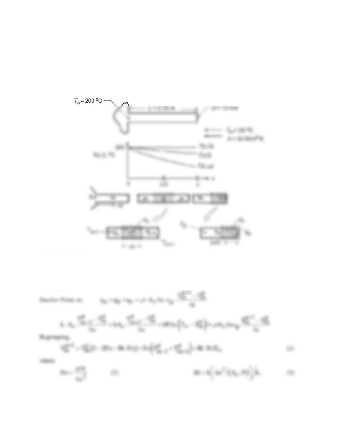
KNOWN: Insulated rod of prescribed length and diameter, with one end in a fixture at 200°C, reaches a

uniform temperature. Suddenly the insulating sleeve is removed and the rod is subjected to a convection

process.

FIND: (a) Time required for the mid-length of the rod to reach 100°C, (b) Temperature history T(x,t ≤

t1), where t1 is time at which the midlength reaches 50°C. Temperature distribution at 0, 200s, 400s and

t1.

SCHEMATIC:

ASSUMPTIONS: (1) One-dimensional transient conduction in rod, (2) Uniform h along rod and at end,

(3) Negligible radiation exchange between rod and surroundings, (4) Constant properties.

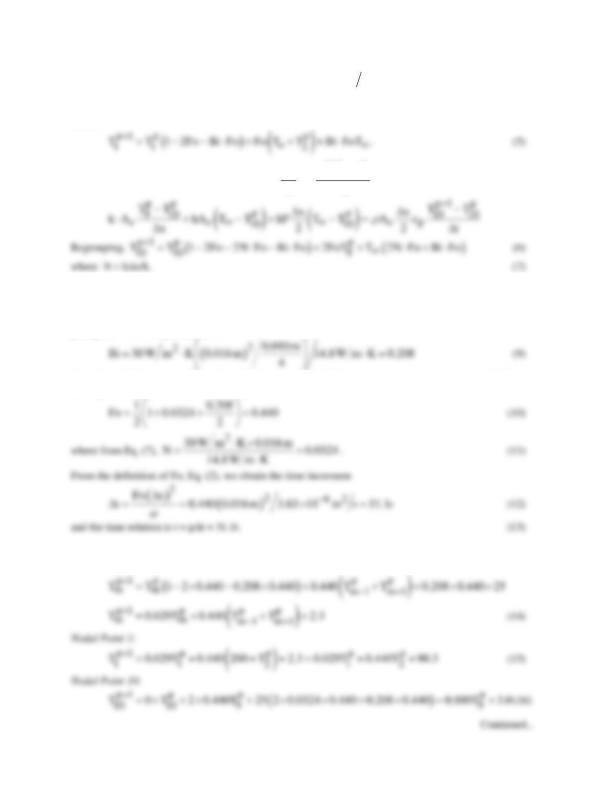
ANALYSIS: (a) Choosing ∆x = 0.016 m, the finite-difference equations for the interior and end nodes

are obtained.

From Eq. (1), recognize that the stability of the numerical solution will be assured when the first term on

the RHS is positive; that is

Continued…

PROBLEM 5.107 (Cont.)

( )

1 2Fo Bi Fo 0− −⋅ ≥

or

( )

Fo12Bi≤+

. (4)

Nodal Point 1: Consider Eq. (1) for the special case that

p

m1

T−

= To, which is independent of time.

Hence,

End Nodal Point 10:

p1 p

10 10

abc c p

TT

x

qqq A c

2t

ρ

+−

∆

++=⋅ ⋅ ∆

The stability criterion is Fo ≤ 1/2(1 + N + Bi/2). (8)

With the finite-difference equations established, we can now proceed with the numerical solution.

Having already specified ∆x = 0.016 m, Bi can now be evaluated. Noting that Ac = πD2/4 and P = πD,

giving Ac/P = D/4, Eq. (3) yields

From the stability criteria, Eqs. (4) and (8), for the finite-difference equations, it is recognized that Eq.

(8) requires the greater value of Fo. Hence

Using the numerical values for Fo, Bi and N, the finite-difference equations can now be written (°C).

Nodal Point m (2 ≤ m ≤ 9):