5.7 Hermite and Hermite Cubic
Interpolation
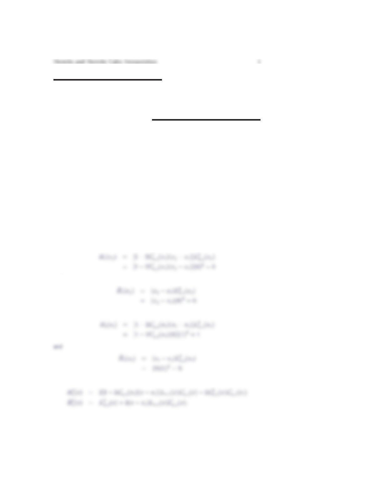
1. Show that the polynomials Hiand ˆ
Hidefined by
Hi(x) = [1 −2L′
n,i(xi)(x−xi)]L2
n,i(x)
ˆ
Hi(x) = (x−xi)L2
n,i(x),
where Ln,i is the Lagrange polynomial associated with the point x=xisatisfy
the relations
Hi(xj) = 1, i =j
0,otherwise ˆ
Hi(xj) = 0
H′
i(xj) = 0 ˆ
H′
i(xj) = 1, i =j
0,otherwise
For i6=j,
and
Morevover,
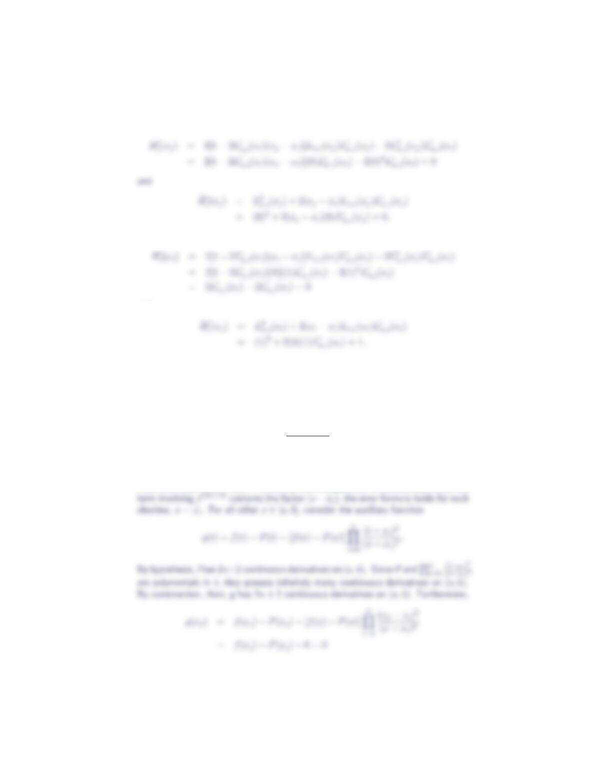
For the derivatives, note that
2Section 5.7
Thus, for i6=j,
Moreover,
and
2. Let fbe continuously differentiable 2n+ 2 times on [a, b], and let x0,x1,x2, …,
xnbe n+ 1 distinct points from [a, b]. Provide the details of the proof that for
each x∈[a, b], there exists a ξ∈[a, b] such that
f(x) = P(x) + f(2n+2)(ξ)
(2n+ 2)!
n
Y
i=0
(x−xi)2,
where Pis the Hermite interpolating polynomial.
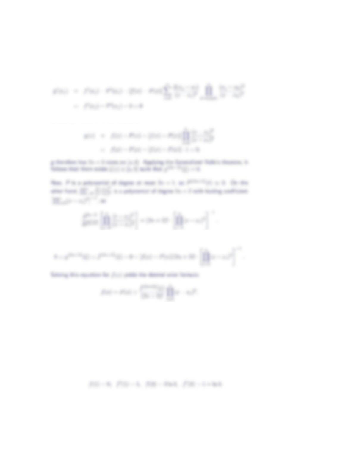
First note that since P(xi) = f(xi)by the interpolation conditions and since the
Hermite and Hermite Cubic Interpolation 3
and
for each j= 0, 1, 2, …, n. Moreover,
Differentiating g2n+ 2 times and evaluating at ξthen gives
3. Let f(x) = xln x,x0= 1 and x1= 3.
(a) Construct the Hermite interpolating polynomial for fat the specified in-
terpolating points.
(b) Approximate f(1.5) using the polynomial from part (a), and confirm that
the theoretical error bound holds.
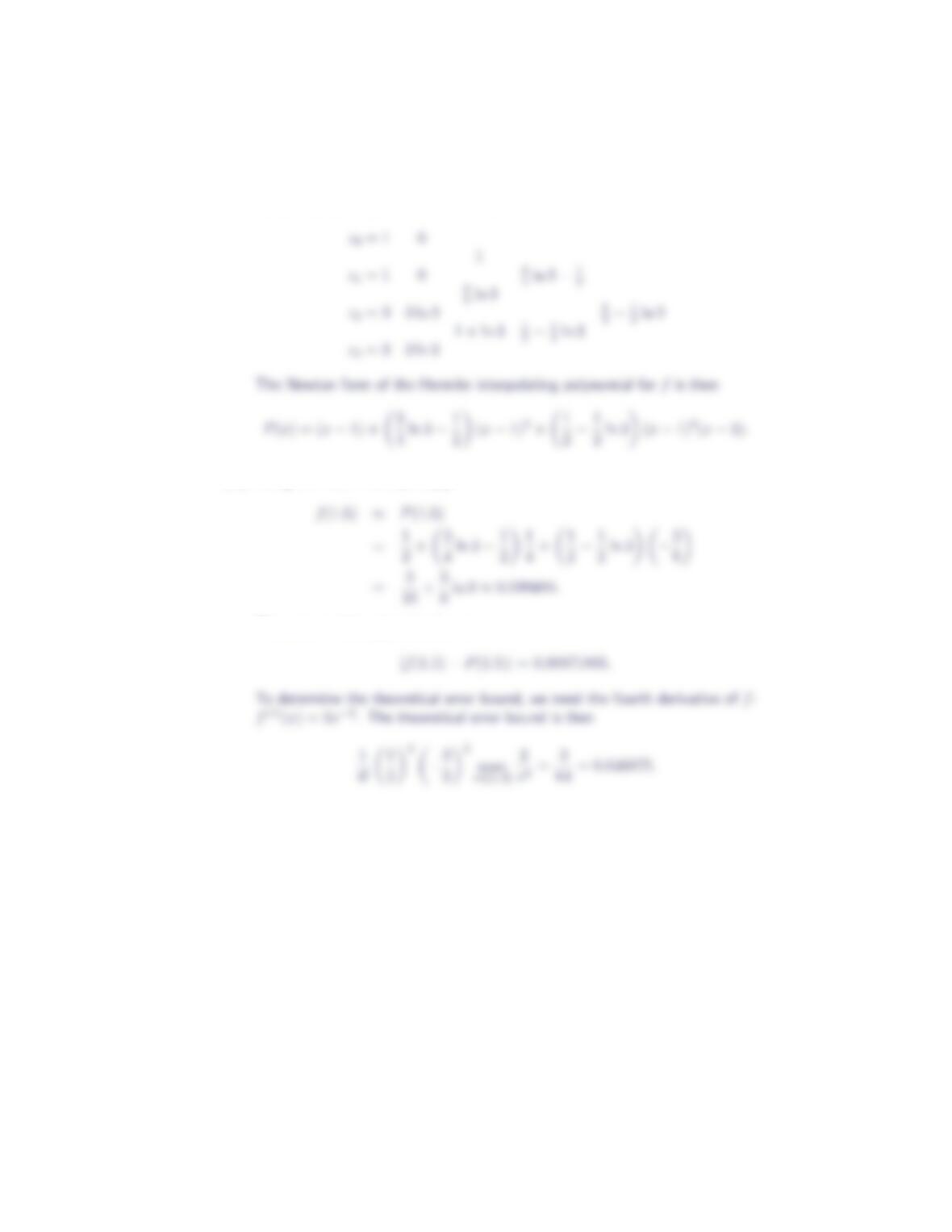
(a) With f(x) = xln x,x0= 1 and x1= 3, we have f′(x) = 1 + ln xand
4Section 5.7
The corresponding divided difference table is
(b) Using the result from part (a),
The error in this approximation is
4. Let f(x) = xln x,x0= 1, x1= 2 and x2= 3.
(a) Construct the Hermite interpolating polynomial for fat the specified in-
terpolating points.
(b) Approximate f(1.5) using the polynomial from part (a), and confirm that
the theoretical error bound holds.
(c) Construct the Hermite cubic interpolant for fat the specified interpolating
points.
(d) Approximate f(1.5) using the piecewise polynomial from part (c), and
confirm that the theoretical error bound holds.
Hermite and Hermite Cubic Interpolation 5
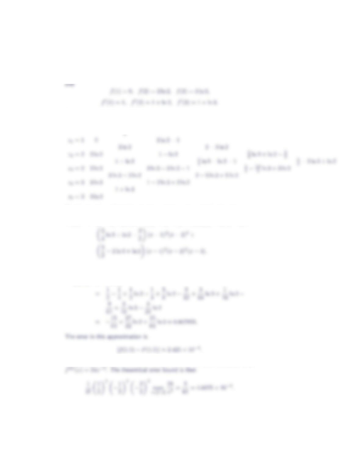
(a) With f(x) = xln x,x0= 1,x1= 2 and x2= 3, we have f′(x) = 1 + ln x
The corresponding divided difference table is
z0= 1 0
The Newton form of the Hermite interpolating polynomial for fis then
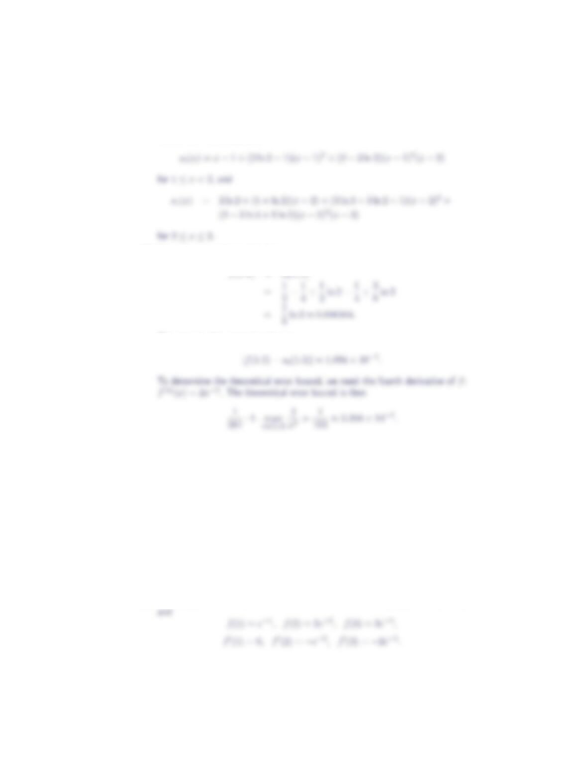
P(x) = (x−1) + (2 ln 2 −1) (x−1)2+ (2 −3 ln 2) (x−1)2(x−2) +
(b) Using the result from part (a),
f(1.5) ≈P(1.5)
To determine the theoretical error bound, we need the sixth derivative of f:
6Section 5.7
(c) Using the divided difference table from (a), we construct the pieces of the
Hermite cubic interpolant:
(d) Using the result from part (c),
f(1.5) ≈s0(1.5)
The error in this approximation is
5. Let f(x) = xe−x,x0= 1, x1= 2 and x2= 3.
(a) Construct the Hermite interpolating polynomial for fat the specified in-
terpolating points.
(b) Approximate f(1.5) using the polynomial from part (a), and confirm that
the theoretical error bound holds.
(c) Construct the Hermite cubic interpolant for fat the specified interpolating
points.
(d) Approximate f(1.5) using the piecewise polynomial from part (c), and
confirm that the theoretical error bound holds.
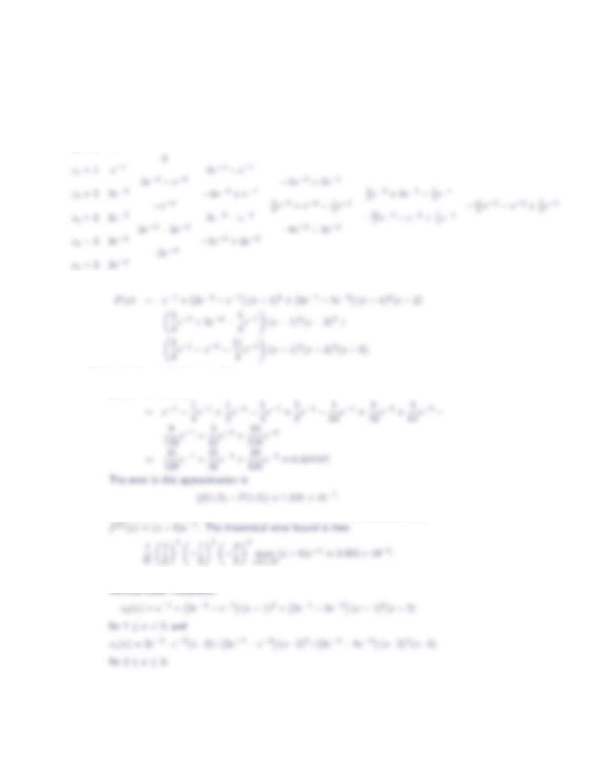
(a) With f(x) = xe−x,x0= 1,x1= 1 and x2= 3, we have f′(x) = e−x(1 −x)
Hermite and Hermite Cubic Interpolation 7
The corresponding divided difference table is
z0= 1 e−1
The Newton form of the Hermite interpolating polynomial for fis then
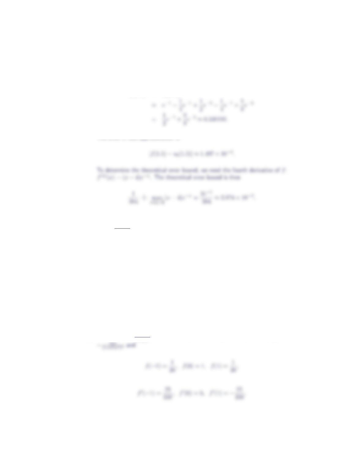
(b) Using the result from part (a),
f(1.5) ≈P(1.5)
To determine the theoretical error bound, we need the sixth derivative of f:
(c) Using the divided difference table from (a), we construct the pieces of the
8Section 5.7
(d) Using the result from part (c),
f(1.5) ≈s0(1.5)
The error in this approximation is
6. Let f(x) = 1
1+25x2,x0=−1, x1= 0 and x2= 1.
(a) Construct the Hermite interpolating polynomial for fat the specified in-
terpolating points.
(b) Approximate f(−0.3) using the polynomial from part (a), and confirm that
the theoretical error bound holds.
(c) Construct the Hermite cubic interpolant for fat the specified interpolating
points.
(d) Approximate f(−0.3) using the piecewise polynomial from part (c), and
confirm that the theoretical error bound holds.
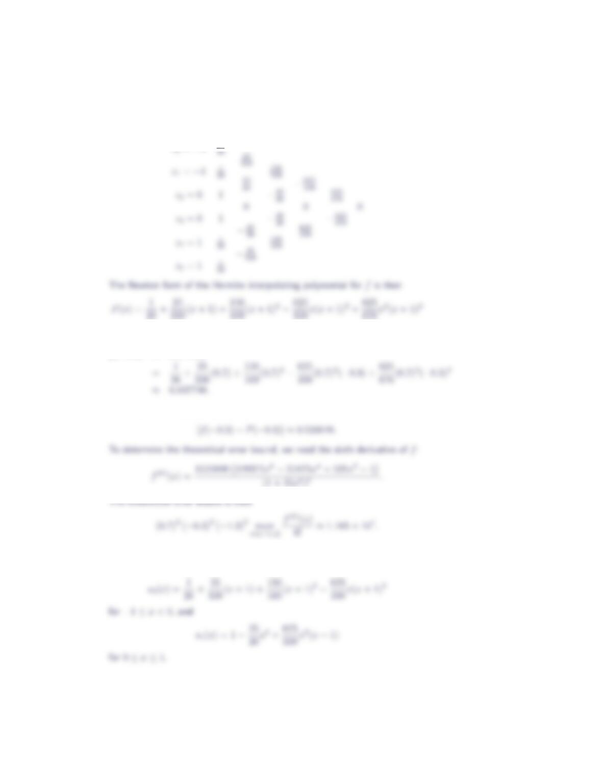
(a) With f(x) = 1
1+25x2,x0=−1,x1= 0 and x2= 1, we have f′(x) =
Hermite and Hermite Cubic Interpolation 9
The corresponding divided difference table is
z0=−11
(b) Using the result from part (a),
f(−0.3) ≈P(−0.3)
The error in this approximation is
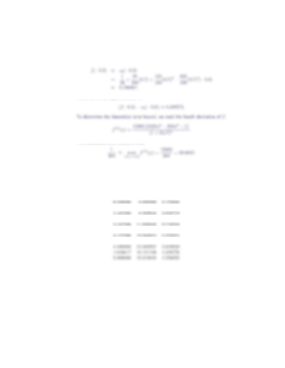
(c) Using the divided difference table from (a), we construct the pieces of the
Hermite cubic interpolant:
10 Section 5.7
(d) Using the result from part (c),
The error in this approximation is
The theoretical error bound is then
7. A model for the growth of an insect population predicts the following values
for the population, P(t), and the rate of increase in the population, P′(t), as
functions of time. Here, time is measured in months.
t P (t)P′(t)
0.000000 5.000000 1.850962
0.950023 7.050280 2.443439
1.947286 9.682456 2.756773
2.947286 12.376723 2.544655
3.947286 14.641031 1.946924
(a) Use the Hermite interpolating polynomial derived from this data to tabu-
late the population in half-week increments.
(b) Use the Hermite cubic interpolating polynomial derived from this data to
tabulate the population in half-week increments.
(c) Use the clamped cubic spline derived from this data to tabulate the pop-
ulation in half-week increments.
(d) Use the not-a-knot cubic spline derived from this data to tabulate the
population in half-week increments.
Hermite and Hermite Cubic Interpolation 11
(e) Compare the results from (a), (b), (c) and (d).
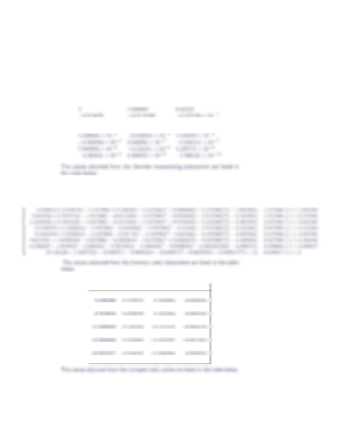
(a) The coefficients of the Newton form of the Hermite interpolating polynomial
are, in order from left to right and from top to bottom,
5.355164 ×10−45.806097 ×10−5−1.337466 ×10⁻⁵
−1.536622 ×10−51.188891 ×10−5−9.116036 ×10⁻⁶
(b) The Hermite cubic interpolant is
5.000000 + 1.850962t+ 0.33122t2−0.010976t2(t−0.5),0≤t < 0.5
6.008286 + 2.179438(t−0.5) + 0.302175(t−0.5)2−0.039358(t−0.5)2(t−0.950023),0.5≤t < 0.950023
7.05028 + 2.443439(t−0.950023) + 0.233365(t−0.950023)2−0.067765(t−0.950023)2(t−1.447286),0.950023 ≤t < 1.447286
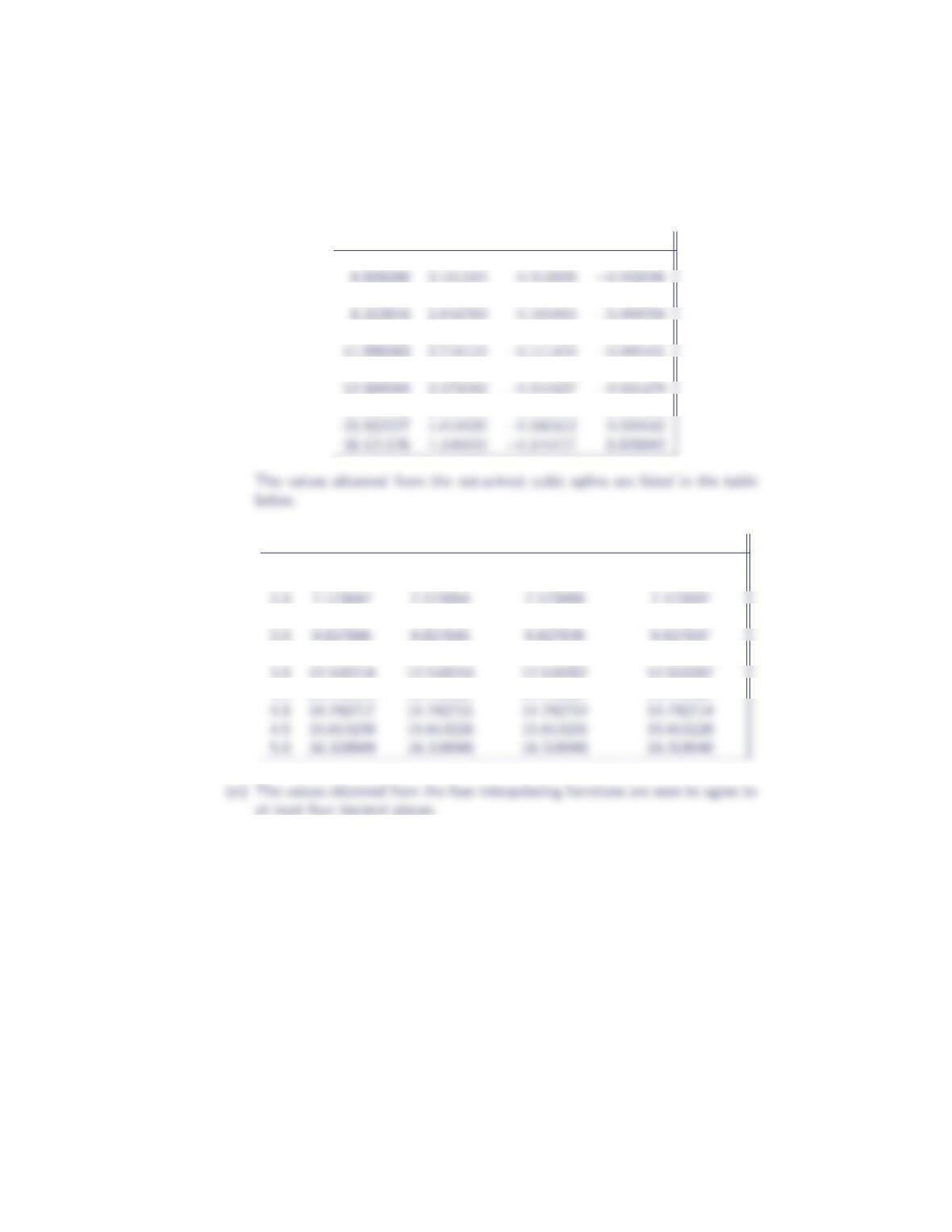
(c) The coefficients of the clamped cubic spline are
ajbjcjdj
5.000000 1.850962 0.336839 −0.011238
7.050280 2.443527 0.266999 −0.067995
9.682456 2.756609 0.030405 −0.094549
12.376723 2.544585 −0.231616 −0.052541
14.641031 1.947008 −0.342683 0.004398
16.121126 1.348822 −0.310587 0.027963
12 Section 5.7
(d) The coefficients of the not-a-knot cubic spline are
ajbjcjdj
5.000000 1.843754 0.361983 −0.032696
7.050280 2.443011 0.268798 −0.069524
9.682456 2.756572 0.030534 −0.094658
12.376723 2.544583 −0.231604 −0.052555
14.641031 1.947016 −0.342655 0.004308
tHermite Hermite Cubic Clamped Cubic Not-a-Knot Cubic
0 5 5 5 5
0.5 6.008286 6.008286 6.008286 6.008286
1.5 8.463611 8.463615 8.463610 8.463616
2.5 11.199410 11.199404 11.199398 11.199399
3.5 13.703535 13.703527 13.703527 13.703527
8. Table 5-1 gives the height and velocity of a free-falling object.
(a) Construct the Hermite cubic interpolant for this data set.
(b) What is the height of the object when t= 0.05 seconds? when t= 0.15
seconds?
(c) At what time is the object 0.20 meters above the ground? 0.10 meters
above the ground?
Hermite and Hermite Cubic Interpolation 13
Table 5-1:
Data for Exercises 8, 9, 10
Time Height Velocity
(sec) (meters) (meters/sec)
0.00 0.290864 −0.16405
0.02 0.284279 −0.32857
0.04 0.274400 −0.49403
0.06 0.260131 −0.71322
0.08 0.241472 −0.93309
0.10 0.219520 −1.09409
0.12 0.189885 −1.47655
0.14 0.160250 −1.47891
0.16 0.126224 −1.69994
0.18 0.086711 −1.96997
0.20 0.045002 −2.07747
0.22 0.000000 −2.25010
Table 5-2:
Data for Exercises 11, 12, 13
Time Charge Current
(sec) (coulombs) (amperes)
0.00 0.000000 0.000000
0.02 0.003293 0.249906
0.04 0.007381 0.121402
0.06 0.007887 −0.053314
0.08 0.006296 −0.080449
0.10 0.005296 −0.015126
0.12 0.005525 0.028800
0.14 0.006086 0.020787
0.16 0.006255 −0.002842
0.18 0.006085 −0.010721
0.20 0.005927 −0.003931
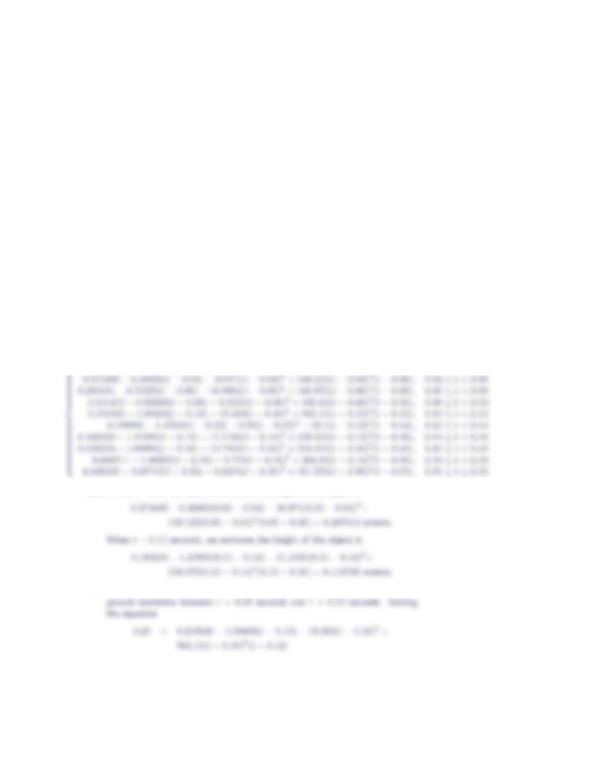
(a) The Hermite cubic interpolant is
0.290864 −0.16405t−8.26t2+ 414.7t2(t−0.02),0.00 ≤t < 0.02
0.284279 −0.32857(t−0.02) −8.269(t−0.02)2+ 413.25(t−0.02)2(t−0.04),0.02 ≤t < 0.04
(b) When t= 0.05 seconds, we estimate the height of the object is
(c) Based on the data, it appears that the object will be 0.20 meters above the