Lagrange Form of the Interpolating Polynomial 1
Solutions
Chapter 5 Interpolation (and Curve Fitting)
5.1 Lagrange Form of the Interpolating
Polynomial
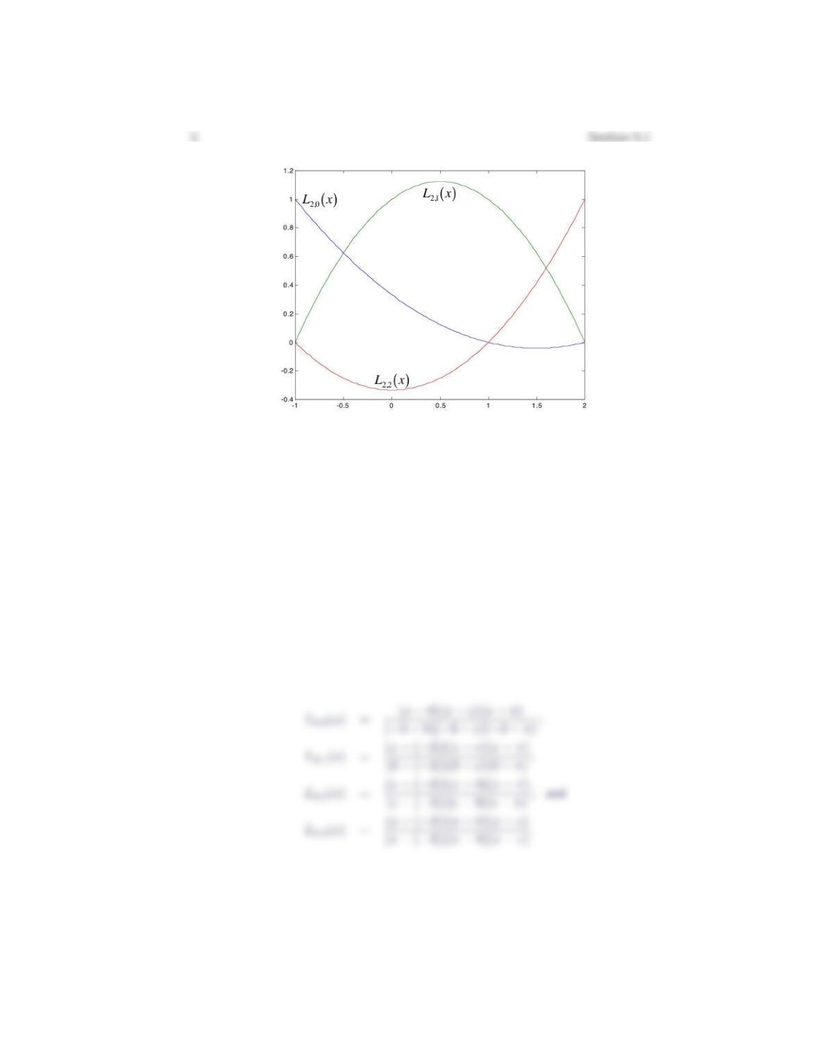
1. Let x0=−1, x1= 1 and x2= 2.
(a) Determine formulas for the Lagrange polynomials L2,0(x), L2,1(x) and
L2,2(x) associated with the given interpolating points.
(b) Plot L2,0(x), L2,1(x) and L2,2(x) on the same set of axes over the range
[−1,2].
(a) With x0=−1,x1= 1 and x2= 2,
2. Let x0=−3, x1= 0, x2=eand x3=π.
(a) Determine formulas for the Lagrange polynomials L3,0(x), L3,1(x), L3,2(x)
and L3,3(x) associated with the given interpolating points.
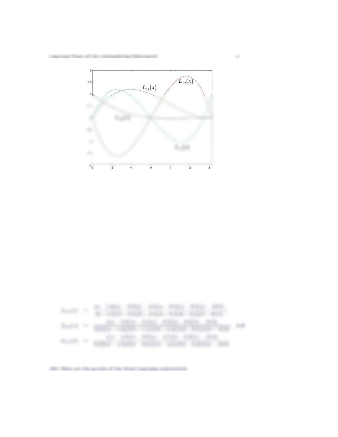
(b) Plot L3,0(x), L3,1(x), L3,2(x) and L3,3(x) on the same set of axes over the
range [−3, π].
(a) With x0=−3,x1= 0,x2=eand x3=π,
(b) Here are the graphs of the four Lagrange polynomials.
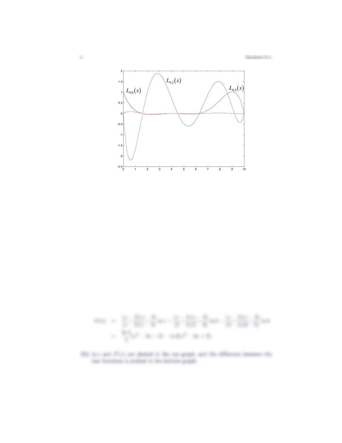
3. Let x0= 0.0, x1= 1.6, x2= 3.8, x3= 4.5, x4= 6.3, x5= 9,2 and x6= 10.0.
(a) Determine formulas for the Lagrange polynomials L6,0(x), L6,2(x) and
L6,5(x) associated with the given interpolating points.
(b) Plot L6,0(x), L6,2(x) and L6,5(x) on the same set of axes over the range
[0,10].
(a) With x0= 0,x1= 1.6,x2= 3.8,x3= 4.5,x4= 6.3,x5= 9.2and
x6= 10.0,
4. Consider the function f(x) = ln x.
(a) Construct the Lagrange form of the interpolating polynomial for fpassing
through the points (1, ln 1), (2, ln 2) and (3, ln 3).
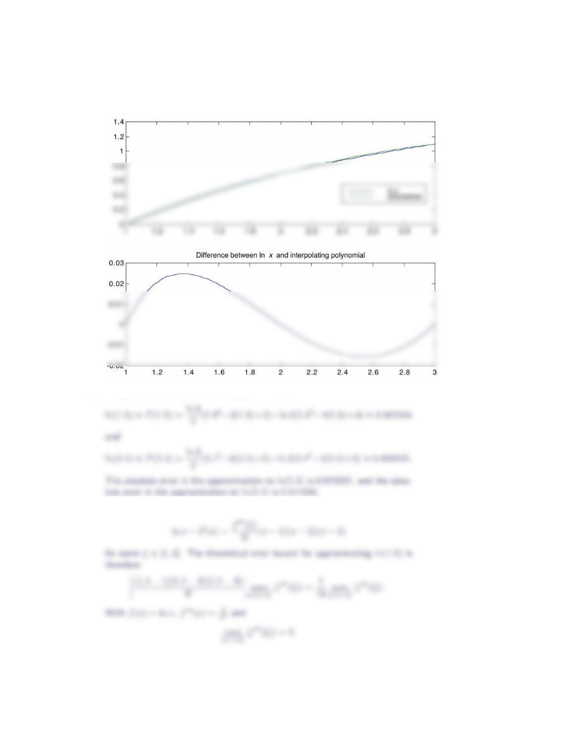
(b) Plot the polynomial obtained in part (a) on the same set of axes as f(x) =
ln x. Use an xrange of [1,3]. Next, generate a plot of the difference
between the polynomial obtained in part (a) and f(x) = ln x.
(c) Use the polynomial obtained in part (a) to estimate both ln(1.5) and
ln(2.4). What is the error in each approximation?
(d) Establish the theoretical error bound for using the polynomial found in
part (a) to approximate ln(1.5). Compare the theoretical error bound to
the error found in part (c).
(a) The Lagrange form of the polynomial passing through the points (1,ln 1),
(2,ln 2) and (3,ln 3) is
Lagrange Form of the Interpolating Polynomial 5
(c) Using the polynomial form part (a), we compute
(d) From the general interpolation error theorem, we know that
6Section 5.1
Thus,
5. Consider the function f(x) = sin x.
(a) Construct the Lagrange form of the interpolating polynomial for fpassing
through the points (0, sin 0), (π/4, sin π/4) and (π/2, sin π/2).
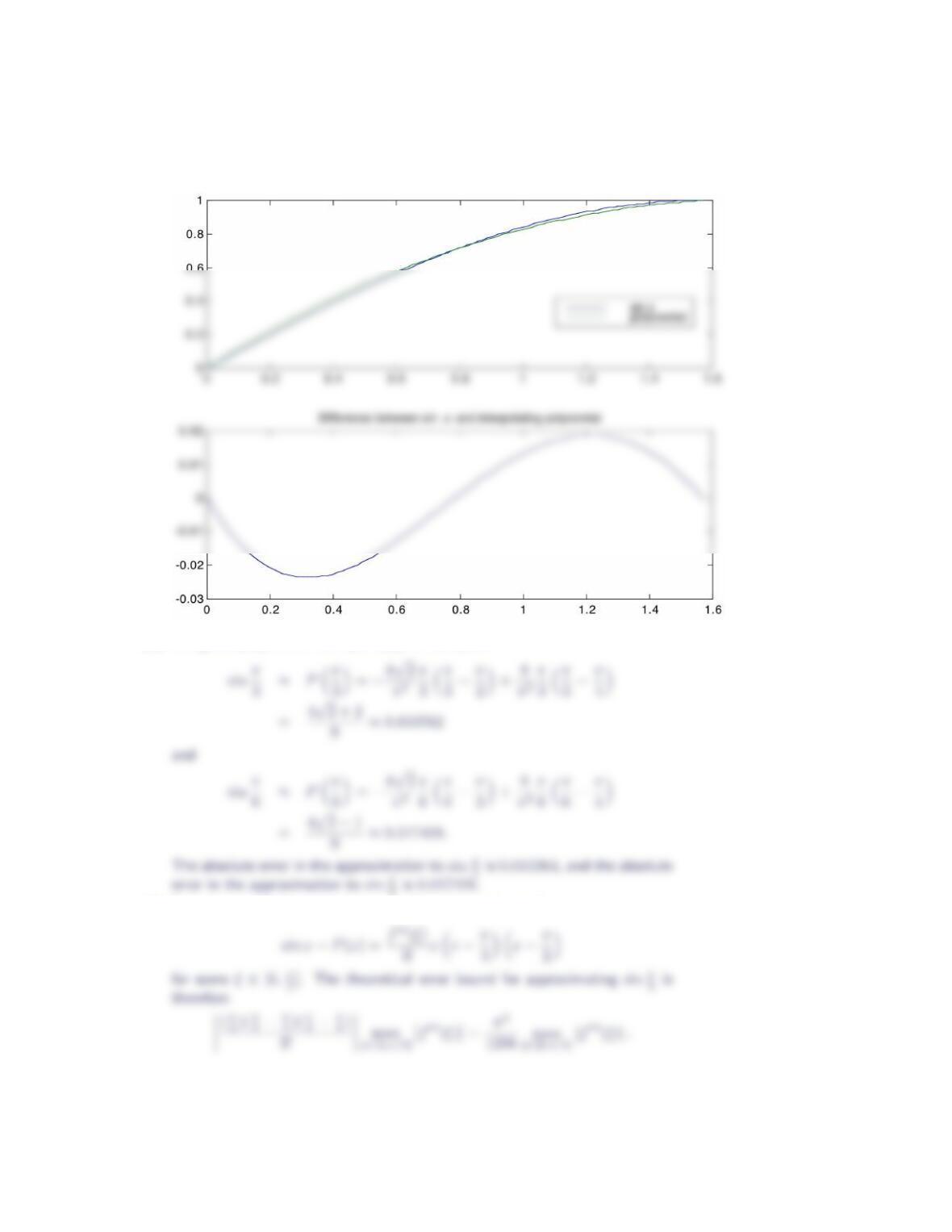
(b) Plot the polynomial obtained in part (a) on the same set of axes as f(x) =
sin x. Use an xrange of [0, π/2]. Next, generate a plot of the difference
between the polynomial obtained in part (a) and f(x) = sin x.
(c) Use the polynomial obtained in part (a) to estimate both sin(π/3) and
sin(π/6). What is the error in each approximation?
(d) Establish the theoretical error bound for using the polynomial found in
part (a) to approximate sin(π/3). Compare the theoretical error bound to
the error found in part (c).
(a) The Lagrange form of the polynomial passing through the points (0,sin 0),
Lagrange Form of the Interpolating Polynomial 7
(c) Using the polynomial from part (a), we compute
(d) From the general interpolation error theorem, we know that
8Section 5.1
With f(x) = sin x,f′′′(x) = −cos xand
6. Consider the function f(x) = ex.
(a) Construct the Lagrange form of the interpolating polynomial for fpassing
through the points (−1, e−1), (0, e0) and (1, e1).
(b) Plot the polynomial obtained in part (a) on the same set of axes as f(x) =
ex. Use an xrange of [−1,1]. Next, generate a plot of the difference
between the polynomial obtained in part (a) and f(x) = ex.
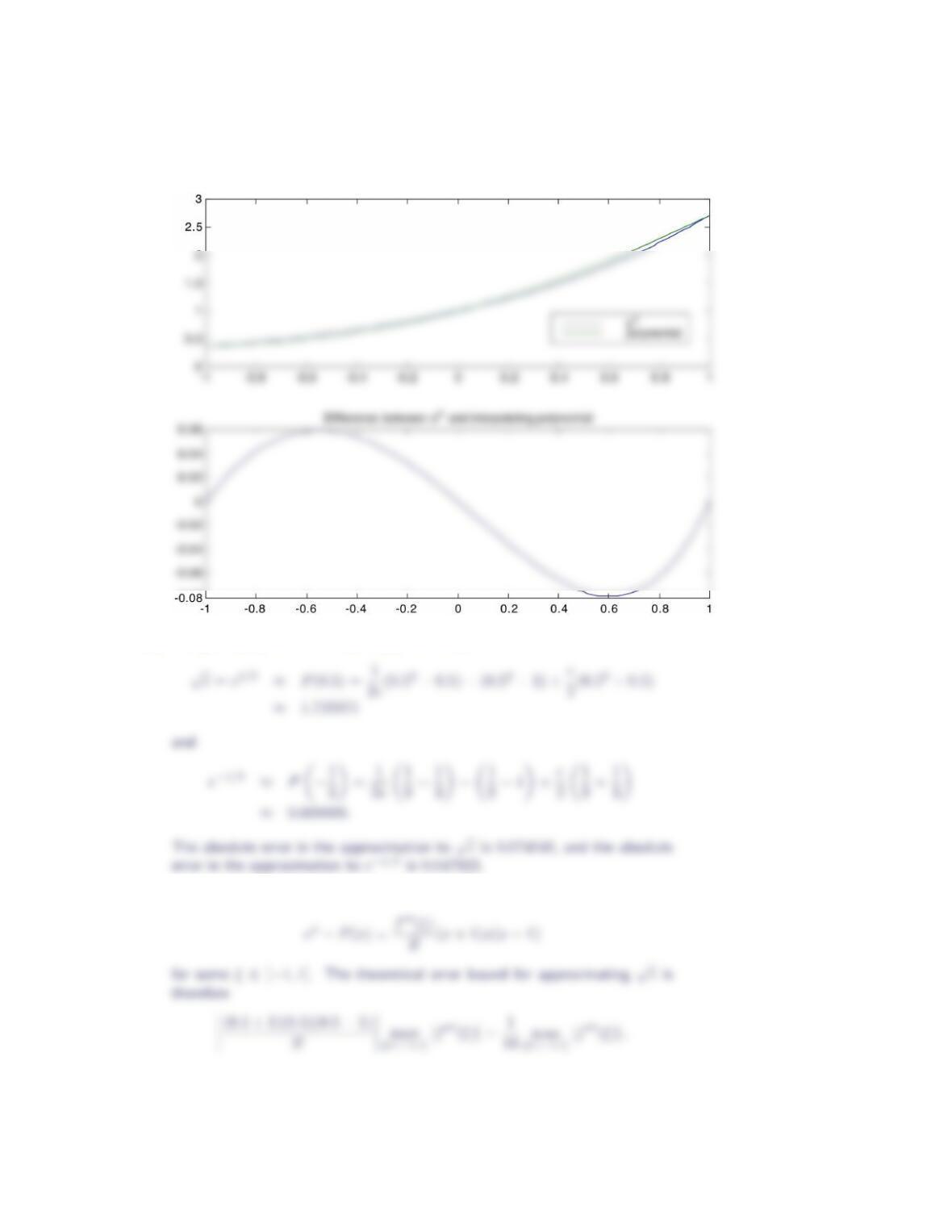
(c) Use the polynomial obtained in part (a) to estimate both √eand e−1/3.
What is the error in each approximation?
(d) Establish the theoretical error bound for using the polynomial found in
part (a) to approximate √e. Compare the theoretical error bound to the
error found in part (c).
(a) The Lagrange form of the polynomial passing through the points (−1, e−1),
(0, e0)and (1, e)is
Lagrange Form of the Interpolating Polynomial 9
(c) Using the polynomial from part (a), we compute
(d) From the general interpolation error theorem, we know that
10 Section 5.1
With f(x) = ex,f′′′(x) = exand
7. Consider the data set
x−1 0 1 2
y5 1 1 11
(a) Show that the polynomials f(x) = x3+ 2x2−3x+ 1 and
g(x) = 1
8x4+3
4x3+15
8x2−11
4x+ 1 both interpolate all of the data.
(b) Why does this not contradict the uniqueness part of the theorem on exis-
tence and uniqueness of polynomial interpolation?
(a) Observe that
f(−1) = −1 + 2 + 3 + 1 = 5;
and
g(−1) = 1
8−3
4+15
8+11
4+ 1 = 40
8= 5;
8. Consider the data set
x−3 1 2 5
y−23 −11 −23 1
Lagrange Form of the Interpolating Polynomial 11
(a) Show that the polynomials f(x) = x3−3x2−10x+ 1 and
g(x) = −23 + 3(x−3) −3(x+ 3)(x−1) + (x+ 3)(x−1)(x−2) both
interpolate all of the data.
(b) Why does this not contradict the uniqueness part of the theorem on exis-
tence and uniqueness of polynomial interpolation?
(a) Observe that
and
(b) Note that
9. Suppose that fis continuous and has continuous first and second derivatives
on the interval [x0, x1]. Derive the following bound on the error due to linear
interpolation of f:
|f(x)−P1(x)| ≤ 1
8h2max
x∈[x0,x1]|f′′(x)|,
where h=x1−x0.
Let P(x)denote the unique linear polynomial that interpolates fat x=x0and
12 Section 5.1
10. The interpolation points influence interpolation error through the polynomial
Πn
i=0(x−xi). Suppose we are interpolating the function fover the interval
[−1,1] using linear interpolation.
(a) If x0=−1 and x1= 1, determine the maximum value of the expression
|(x−x0)(x−x1)|for −1≤x≤1.
(b) If x0=−√2/2 and x1=√2/2, determine the maximum value of the
expression |(x−x0)(x−x1)|for −1≤x≤1. How does this compare to
the maximum found in part (a)?
(c) Select any two numbers from the interval [−1,1] to serve as the interpo-
lation points x0and x1. Determine the maximum value of the expression
|(x−x0)(x−x1)|for −1≤x≤1, and compare to the maxima found in
parts (a) and (b).
(a) With x0=−1and x1= 1,|(x−x0)(x−x1)|=|x2−1|. Since x2−1≤0
(b) With x0=−√2
11. The interpolation points influence interpolation error through the polynomial
Πn
i=0(x−xi). Suppose we are interpolating the function fover the interval
[−1,1] using quadratic interpolation.
(a) If x0=−1, x1= 0 and x2= 1, determine the maximum value of the
expression |(x−x0)(x−x1)(x−x2)|for −1≤x≤1.
(b) If x0=−√3/2, x1= 0 and x2=√3/2, determine the maximum value of
the expression |(x−x0)(x−x1)(x−x2)|for −1≤x≤1. How does this
compare to the maximum found in part (a)?
(c) Select any three numbers from the interval [−1,1] to serve as the interpola-
tion points x0,x1and x2. Determine the maximum value of the expression
|(x−x0)(x−x1)(x−x2)|for −1≤x≤1, and compare to the maxima
found in parts (a) and (b).
(b) With x0=−√3
12. The following data set was taken from a polynomial of degree at most five. Find
the polynomial.
x−2−10123
y39 3 −1−3−9−1
14 Section 5.1
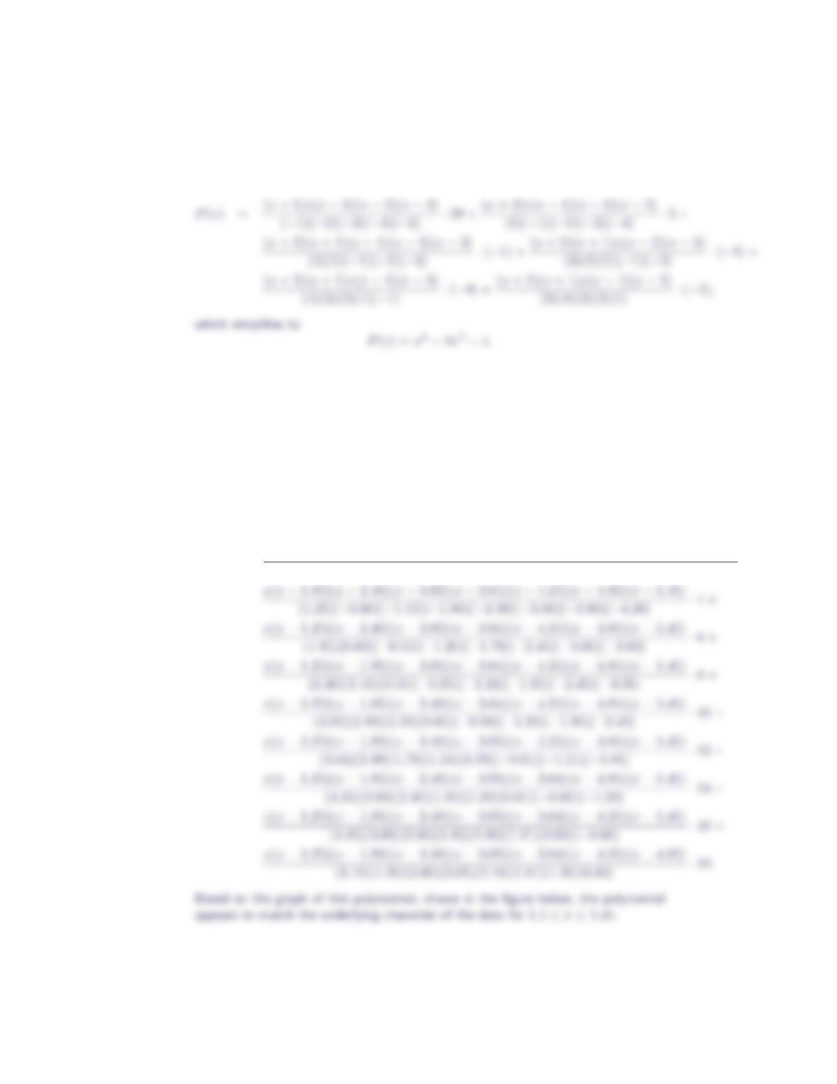
The Lagrange form of the interpolating polynomial is
13. Consider the data set
x0 1.25 1.85 2.40 3.05 3.64 4.25 4.85 5.45
y0 4 6 8 10 12 14 16 18
Determine the polynomial of degree at most eight (8) which interpolates this
data. Over what range of xvalues would you feel comfortable using the inter-
polating polynomial to approximate values of y? Explain.
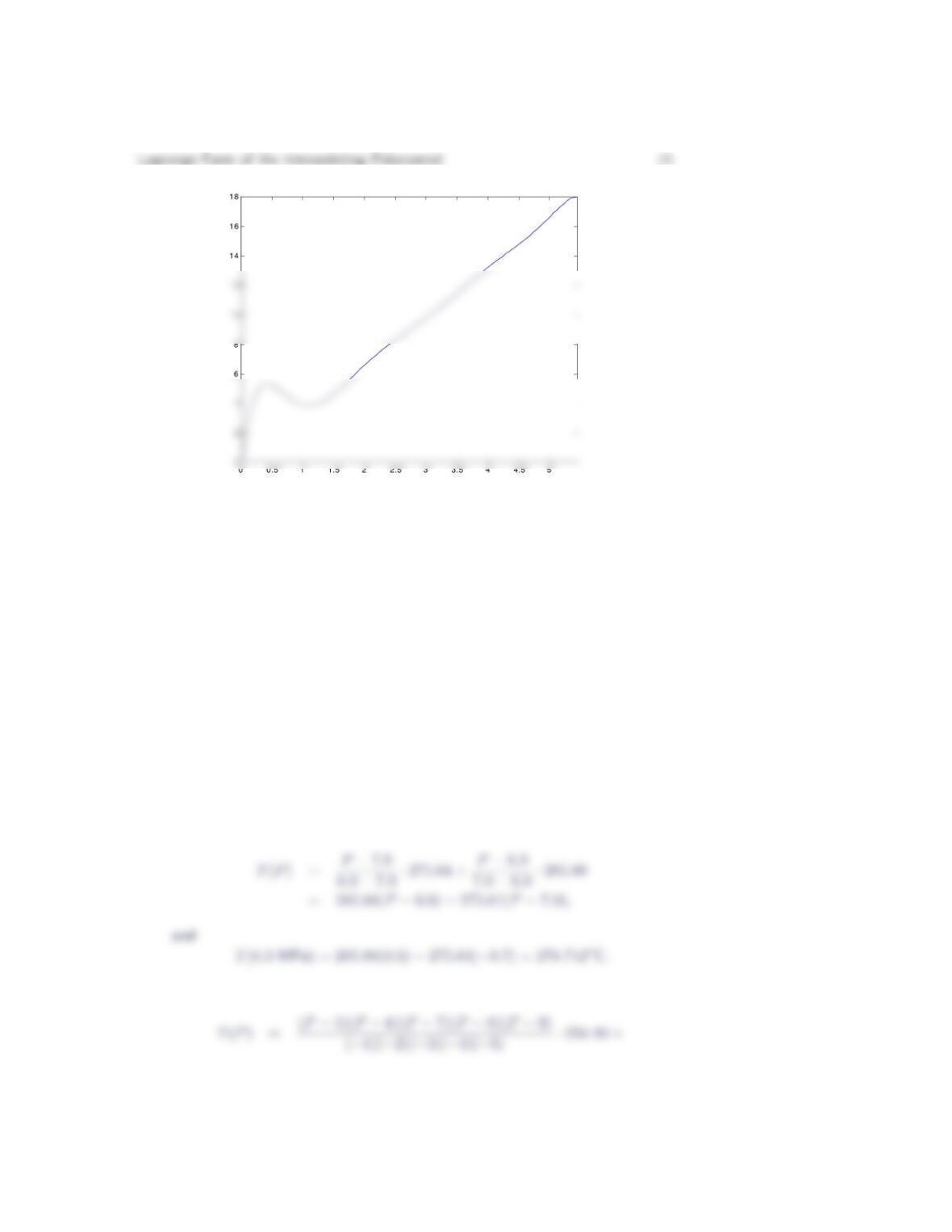
The Lagrange form of the interpolating polynomial is
P(x) = (x−1.25)(x−1.85)(x−2.40)(x−3.05)(x−3.64)(x−4.25)(x−4.85)(x−5.45)
(−1.25)(−1.85)(−2.40)(−3.05)(−3.64)(−4.25)(−4.85)(−5.45) ·0 +
14. A thermodynamics student needs the temperature of saturated steam under a
pressure of 6.3 mega-Pascals (MPa).
(a) Estimate the temperature using linear interpolation from the data
Pressure (MPa) Temperature (◦C)
6.0 275.64
7.0 285.88
(b) Estimate the temperature using polynomial interpolation from the data
Pressure (MPa) 4.0 5.0 6.0 7.0 8.0 9.0
Temperature (◦C) 250.40 263.99 275.64 285.88 295.06 303.40
(c) Which approximation do you think is more accurate and why?
(a) Let Tdenote the temperature and Pdenote the pressure of saturated steam.
Using the given data,
(b) Using the given data,
16 Section 5.1
(P−4)(P−6)(P−7)(P−8)(P−9)
(1)(−1)(−2)(−3)(−4) ·263.99 +
and T(6.3MPa) = 278.841◦C.
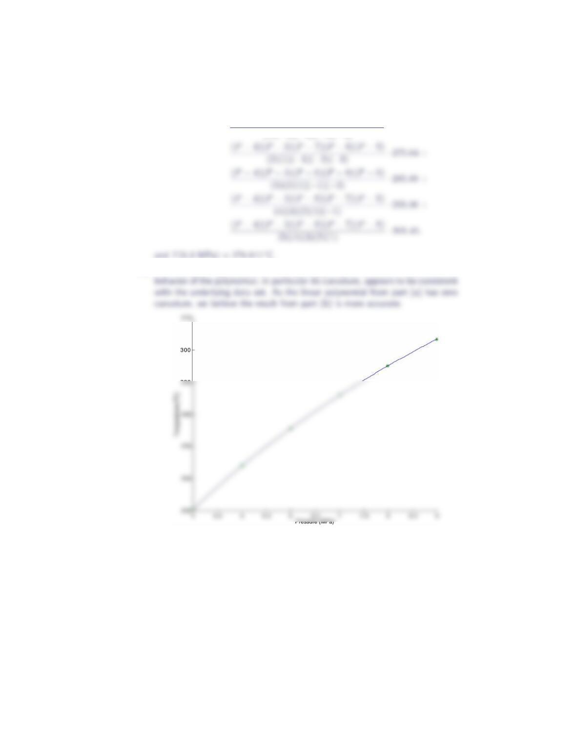
(c) The interpolating polynomial from part (b) is plotted below. Note that the
15. Perry’s Chemical Engineer’s Handbook gives the following values for the heat
capacity at constant pressure, cp, of an aqueous solution of methyl alcohol as a
function of the alcohol mole percentage, φ:
φ(%) 5.88 12.3 27.3 45.8 69.6 100.0
cp(cal/g ◦C) 0.995 0.98 0.92 0.83 0.726 0.617
All data is provided at T= 40◦Cand atmospheric pressure. A table which lists
the heat capacity at constant pressure for φ= 5, 10, 15, …, 100% is desired.
Lagrange Form of the Interpolating Polynomial 17
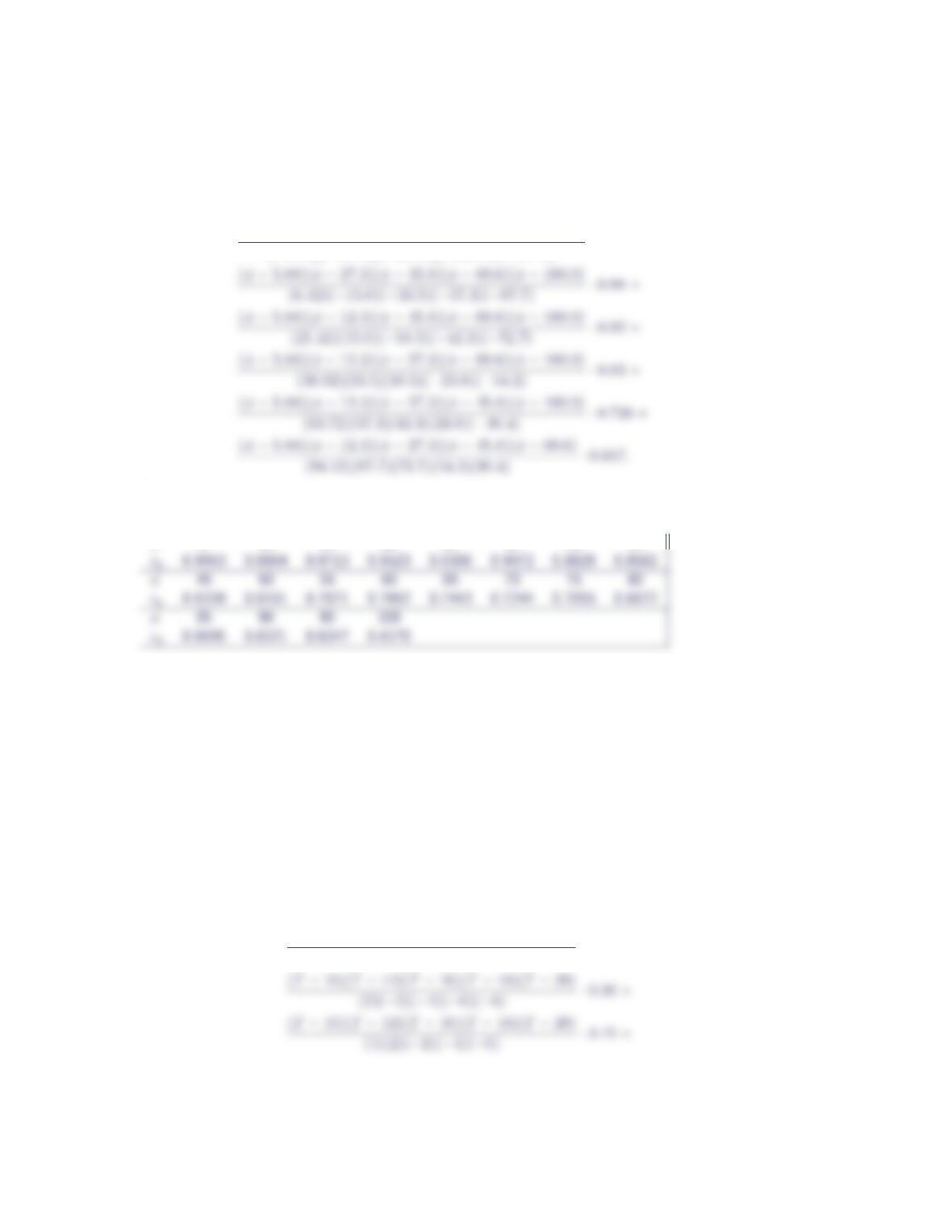
The Lagrange form of the interpolating polynomial is
cp(φ) = (φ−12.3)(φ−27.3)(φ−45.8)(φ−69.6)(φ−100.0)
(−6.42)(−21.42)(−39.92)(−63.72)(−94.12) ·0.995 +
Evaluating this polynomial for φ= 5,10,15,…,100% produces the values given in
the following table.
φ5 10 15 20 25 30 35 40
16. The table below lists the linewidth of a printed feature on a semiconductor
device as a function of the dissolution time (the amount of time the silicon
wafer is placed in the developer solution).
Dissolution Time (sec) 10 12 14 16 18 20
Linewidth (µm) 0.25 0.36 0.45 0.50 0.53 0.55
(a) Approximate the linewidth of the feature after a dissolution time of 15
seconds.
(b) Plot the values in the table, together with the value obtained in part (a).
Does the result from part (a) seem reasonable? Explain.
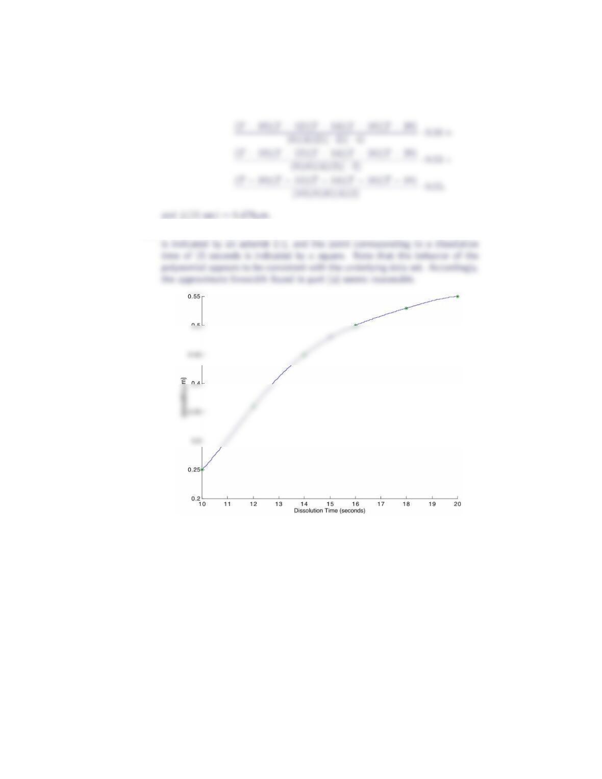
(a) Let Ldenote the linewidth and Tdenote the dissolution time. Then
L(T) = (T−12)(T−14)(T−16)(T−18)(T−20)
(−2)(−4)(−6)(−8)(−10) ·0.25 +
18 Section 5.1
(b) The interpolating polynomial from part (a) is plotted below. Each data point
17. The following table gives the viscosity, in millipascal-seconds (centipoises) of
sulfuric acid as a function of concentration, in mass percent.
concentration 0 20 40 60 80 100
viscosity 0.89 1.40 2.51 5.37 17.4 24.2
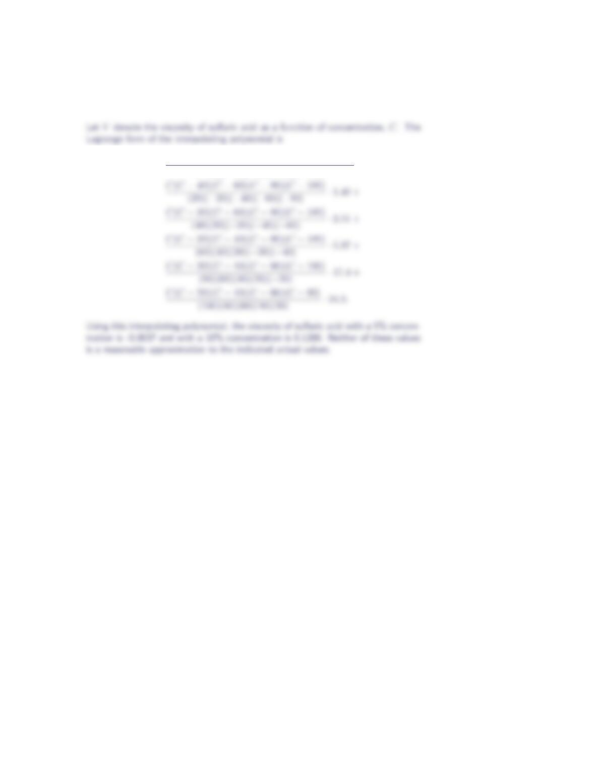
Determine the polynomial of degree at most five which interpolates this data.
The viscosity of sulfuric acid with a 5% concentration is 1.01 and with a 10%
concentration is 1.12. Use these values to assess the accuracy of the interpolating
polynomial.
Lagrange Form of the Interpolating Polynomial 19
V(C) = (C−20)(C−40)(C−60)(C−80)(C−100)
(−20)(−40)(−60)(−80)(−100) ·0.89 +