5.3 Newton Form of the Interpolating
Polynomial
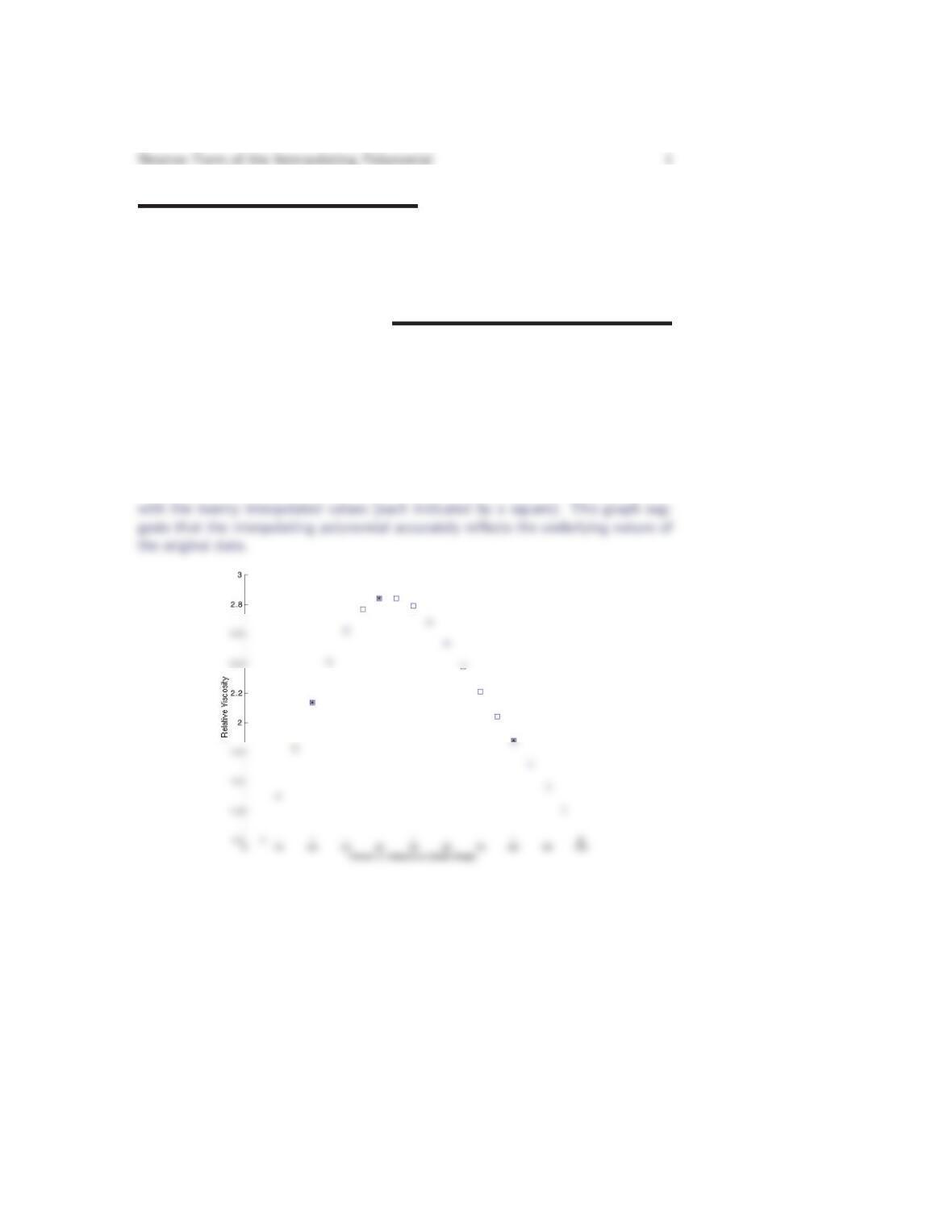
1. Assess the accuracy of the values in the relative viscosity table developed earlier
in this section by plotting the values from the table and the six given data values
on the same set of axes.
The graph below shows all six data points (each indicated by an asterisk) together
2. A more extensive table lists the viscosity of ethanol as 2.209 when the anhydrous
solute weight is 70%. Add this value to the bottom of the divided difference
table provided in the example in the text and compute the new values at the
bottom of each column. What is the interpolating polynomial using seven data
points rather than the original six?
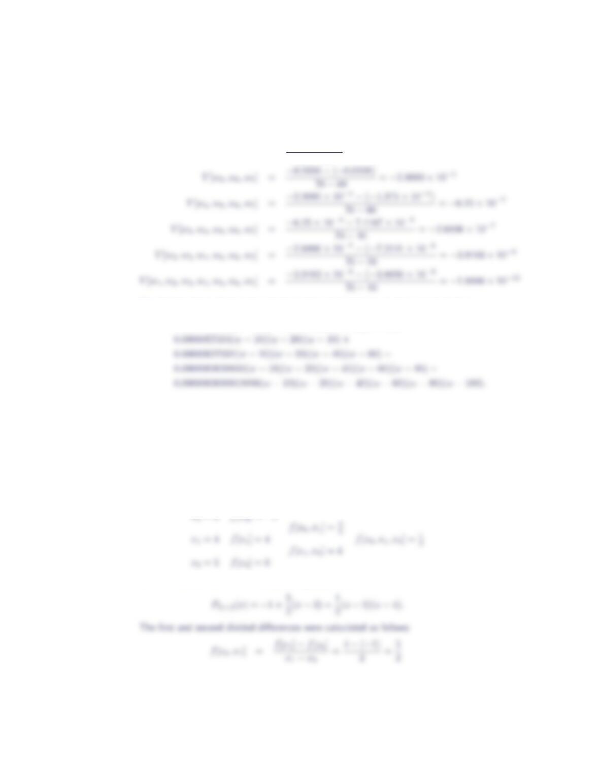
Including the new data point (70,2.209) at the bottom of the original divided
difference table, we calculate the following values along the bottom diagonal of the
2Section 5.3
augmented table:
V[w6, w7] = 2.209 −1.201
70 −100 =−0.0336
The Newton form of the interpolating polynomial using seven data points is then
V= 1.498 + 0.064(w−10) −0.00096333(w−10)(w−20) −
3. Construct the divided difference table for the following data set, and then write
out the Newton form of the interpolating polynomial.
x2 4 5
y−148
The complete divided difference table is
and the Newton form of the interpolating polynomial is

Newton Form of the Interpolating Polynomial 3
4. Construct the divided difference table for the following data set, and then write
out the Newton form of the interpolating polynomial.
x0 1 2
y2−1 4
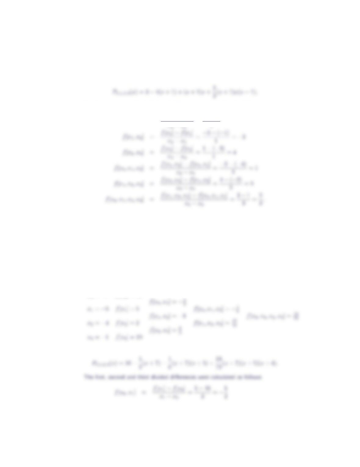
The complete divided difference table is
x0= 0 f[x0] = 2
and the Newton form of the interpolating polynomial is
The first and second divided differences were calculated as follows:
5. Construct the divided difference table for the following data set, and then write
out the Newton form of the interpolating polynomial.
x−1 0 1 2
y3−1−3 1
The complete divided difference table is
x0=−1f[x0] = 3
4Section 5.3
and the Newton form of the interpolating polynomial is
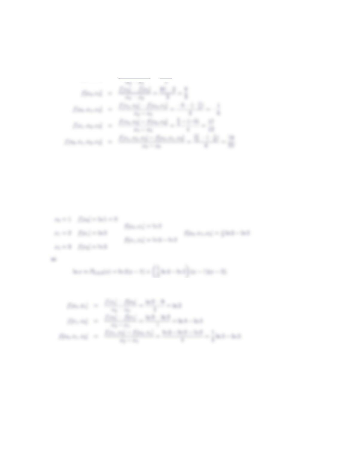
The first, second and third divided differences were calculated as follows:
f[x0, x1] = f[x1]−f[x0]
x1−x0
=−1−3
1=−4
6. Construct the divided difference table for the following data set, and then write
out the Newton form of the interpolating polynomial.
x−7−5−4−1
y10 5 2 10
The complete divided difference table is
x0=−7f[x0] = 10
and the Newton form of the interpolating polynomial is
Newton Form of the Interpolating Polynomial 5
f[x1, x2] = f[x2]−f[x1]
=2−5
7. Write out the Newton form of the interpolating polynomial for f(x) = ln x
which passes through the points (1,ln 1), (2,ln 2) and (3,ln 3).
The complete divided difference table is
The first and second divided differences were calculated as follows:
8. Write out the Newton form of the interpolating polynomial for f(x) = sin x
which passes through the points (0,sin 0), (π/4,sin π/4) and (π/2,sin π/2).
The complete divided difference table is
6Section 5.3
x0= 0 f[x0] = sin 0 = 0
The first and second divided differences were calculated as follows:
9. Write out the Newton form of the interpolating polynomial for f(x) = exwhich
passes through the points (−1, e−1), (0, e0) and (1, e1).
The complete divided difference table is
x0=−1f[x0] = e−1
2(x+ 1)x.
The first and second divided differences were calculated as follows:
f[x0, x1] = f[x1]−f[x0]
=1−e−1
10. Determine the missing values in the divided difference table provided below.
Newton Form of the Interpolating Polynomial 7
x0= 0 f[x0] = −1
f[x0, x1] = 5
x1= 1 f[x1] =? f[x0, x1, x2] = −3
2
f[x1, x2] =?
x2= 2 f[x2] =?
From
f[x0, x1] = f[x1]−f[x0]
x1−x0
we have 5 = f[x1]−(−1)
1−0,
11. Determine the missing values in the divided difference table provided below.
x0= 0 f[x0] = 1
f[x0, x1] = 2
x1= 1 f[x1] = 3 f[x0, x1, x2] =?
f[x1, x2] =? f[x0, x1, x2, x3] =?
x2= 2 f[x2] = 3 f[x1, x2, x3] = 0
f[x2, x3] = 0
x3= 3 f[x3] =?
Knowing f[x1] = f[x2] = 3, we find
f[x1, x2] = f[x2]−f[x1]
=3−3
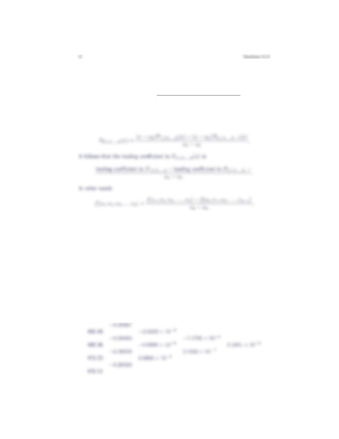
12. Let f[x0, x1, x2, …, xk] be defined as the leading coefficient in the unique poly-
nomial which interpolates fat the points x0,x1,x2, …, xk. Show that
f[x0, x1, x2, …, xk] = f[x1, x2, …, xk]−f[x0, x1, …, xk−1]
xk−x0
.
Let f[x0, x1, x2,…,xk]be the leading coefficient in the unique polynomial inter-
polating fat the points x0, x1, x2,…,xk. From the formula
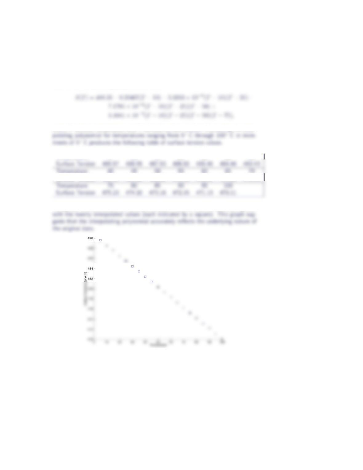
13. The values listed in the table provide the surface tension of mercury as a function
of temperature.
Temperature (◦C) 10 25 50 75 100
Surface Tension (dyn/cm) 488.55 485.48 480.36 475.23 470.11
Use these values to determine the Newton form of the interpolating polynomial,
and then use the polynomial to produce a table of surface tension values for
temperatures ranging from 5◦C through 100◦C in increments of 5◦C. Assess the
accuracy of the table by plotting the values from the table and the five given
data values on the same set of axes.
The complete divided difference table is
488.55
Newton Form of the Interpolating Polynomial 9
where all values have been rounded to five digits for display purposes. The Newton
form of the interpolating polynomial is then
where Tdenotes temperature and Sdenotes surface tension. Evaluating the inter-
Temperature 5 10 15 20 25 30 35
Surface Tension 482.41 481.38 480.36 479.33 478.31 477.28 476.25
The graph below shows all five data points (each indicated by an asterisk) together
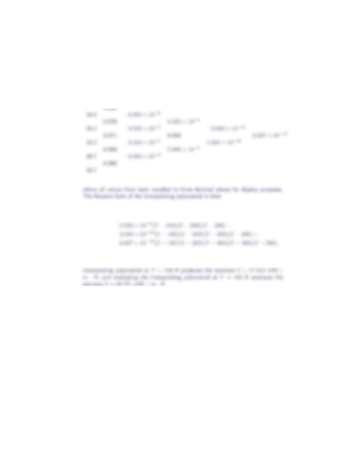
14. The thermal conductivity of air as a function of temperature is given in the
table below. Estimate the thermal conductivity of air when T=240K and when
T=485K, using the Newton form of the interpolating polynomial.
Temperature (K) 100 200 300 400 500 600
Thermal Conductivity (mW/m·K) 9.4 18.4 26.2 33.3 39.7 45.7
10 Section 5.3
The complete divided difference table is
9.4
k(T) = 9.4−0.090(T−100) −6.000 ×10⁻⁵(T−100)(T−200)+
where Tdenotes temperature and kdenotes thermal conductivity. Evaluating the
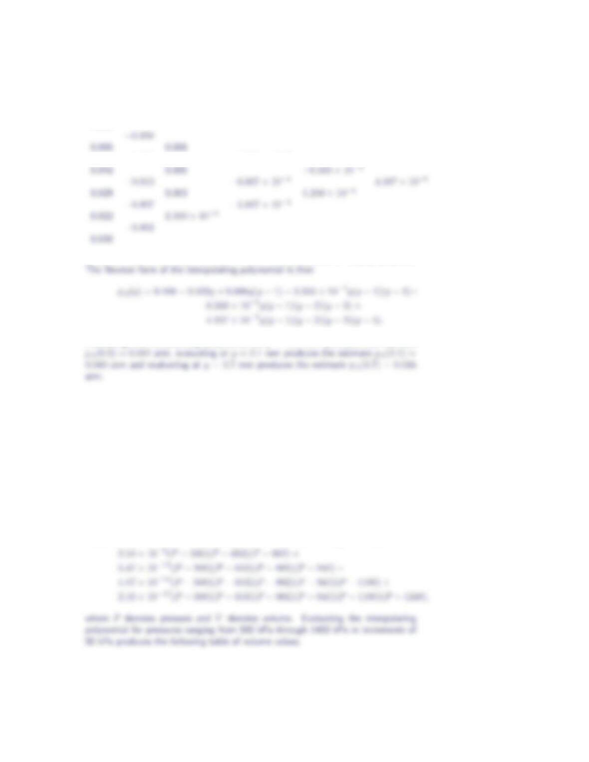
15. Experimentally determined values for the partial pressure of water vapor, pA,
as a function of distance, y, from the surface of a pan of water are given below.
Estimate the partial pressure at distances of 0.5 mm, 2.1 mm and 3.7 mm from
the surface of the water.
y(mm) 0 1 2 3 4 5
pA(atm) 0.100 0.065 0.042 0.029 0.022 0.020
The complete divided difference table is
Newton Form of the Interpolating Polynomial 11
0.100
−0.023 −3.333 ×10⁻⁴
where all values have been rounded to three decimal places for display purposes.
Evaluating the interpolating polynomial at y= 0.5mm produces the estimate
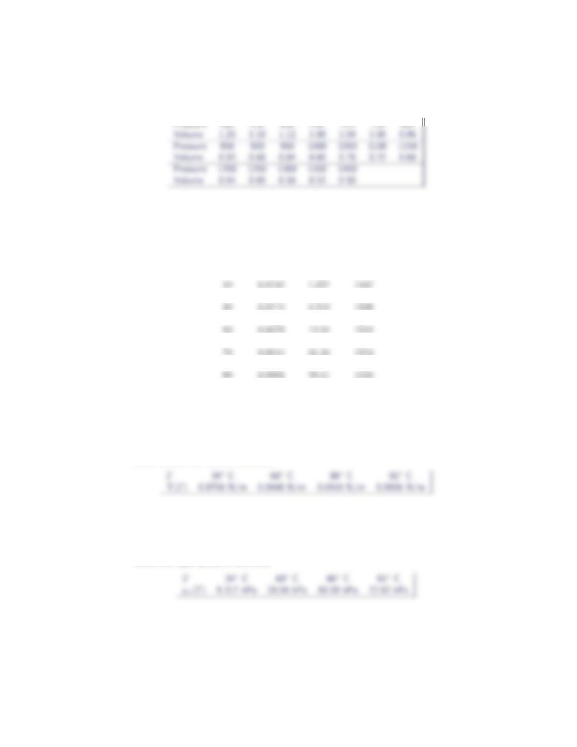
16. Ammonia vapor is compressed inside a cylinder by an external force acting on
the piston. The ammonia is initially at 30◦C, 500 kPa and the final pressure is
1400 kPa. The following data have been experimentally determined during the
process. Use the Newton form of the interpolating polynomial to determine a
table of volume as a function of pressure, with pressure ranging from 500 kPa
through 1400 kPa in increments of 50 kPa.
Pressure (kPa) 500 653 802 945 1100 1248 1400
Volume (l) 1.25 1.08 0.96 0.84 0.72 0.60 0.50
The Newton form of the interpolating polynomial is
V(P) = 1.25 −1.11 ×10⁻³(P−500) + 1.01 ×10⁻⁶(P−500)(P−653)−
12 Section 5.3
Table A.5 in Frank White, Fluid Mechanics, lists the following values for the sur-
face tension, Υ, vapor pressure, pv, and sound speed, a, for water as a function
of temperature. Use this data for Exercises 17 – 19.
T (◦C) Υ (N/m) pv(kPa) a(m/s)
0 0.0756 0.611 1402
20 0.0728 2.337 1482
40 0.0696 7.375 1529
60 0.0662 19.92 1551
80 0.0626 47.35 1554
100 0.0589 101.3 1543
17. Use the Newton form of the interpolating polynomial to determine the surface
tension of water when T = 34◦C, 68◦C, 86◦C and 91◦C.
Evaluating the interpolating polynomial at the indicated temperature values pro-
duces the surface tension estimates
18. Use the Newton form of the interpolating polynomial to determine the vapor
pressure of water when T = 34◦C, 68◦C, 86◦C and 91◦C.
Evaluating the interpolating polynomial at the indicated temperature values pro-
duces the vapor pressure estimates
19. Use the Newton form of the interpolating polynomial to determine the sound
speed of water when T = 34◦C, 68◦C, 86◦C and 91◦C.

Newton Form of the Interpolating Polynomial 13