Cubic Spline Interpolation 1
5.6 Cubic Spline Interpolation
For Exercises 1 through 3, use the values given below for the temperature, T,
pressure, p, and density, ρ, of the standard atmosphere as a function of altitude.
This data was drawn from Table A.6 in Frank White, Fluid Mechanics:
z(m) 0 500 1000 1500 2000 2500 3000
T(K) 288.16 284.91 281.66 278.41 275.16 271.91 268.66
p(Pa) 101,350 95,480 89,889 84,565 79,500 74,684 70,107
ρ(kg/m3) 1.2255 1.1677 1.1120 1.0583 1.0067 0.9570 0.9092
1. Using the not-a-knot cubic spline interpolant, estimate the temperature of the
standard atmosphere at an altitude of z= 800 m, 1600 m, 2350 m and 2790 m?
At what altitude is the temperature of the standard atmosphere 273.1 K?
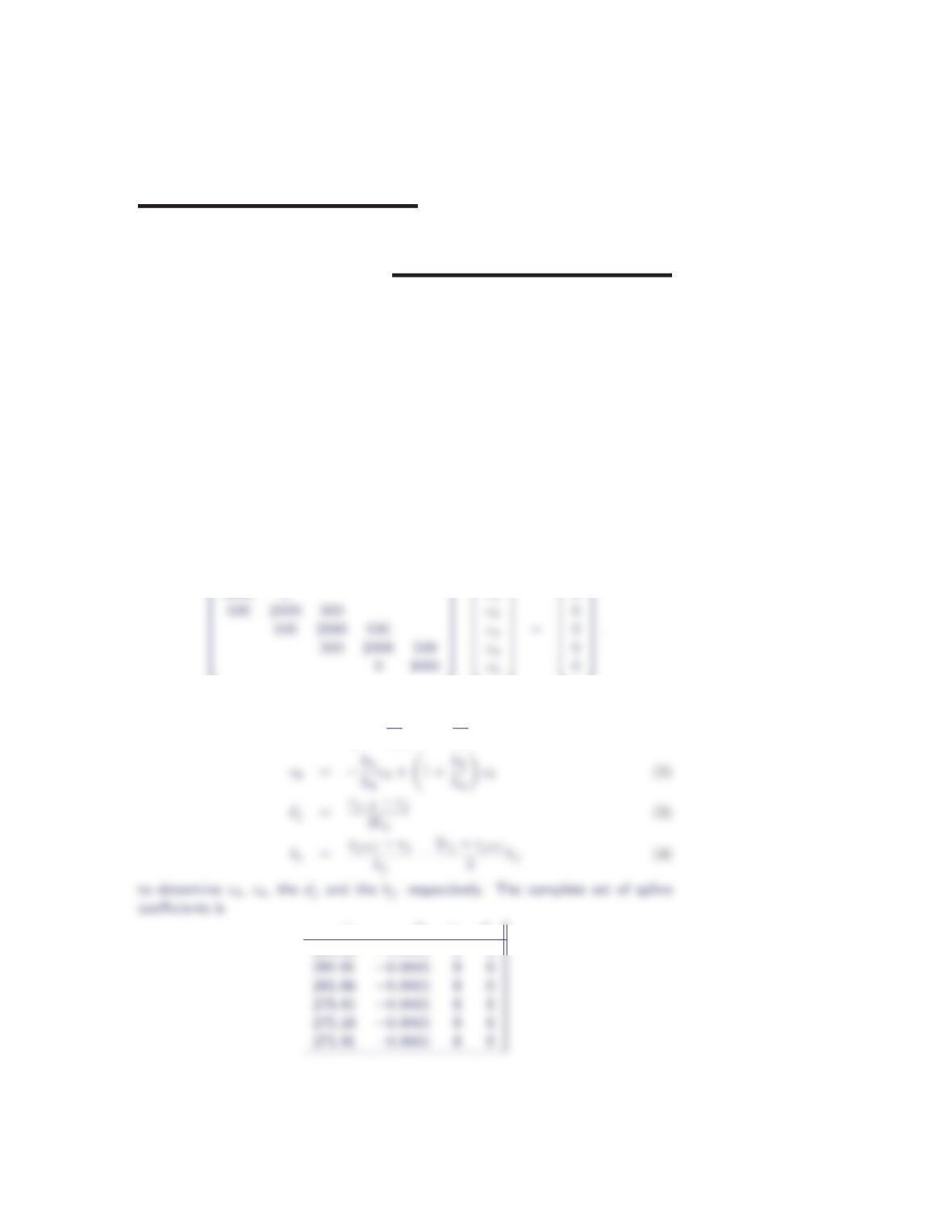
The linear system for the coefficients cj(1≤j≤5) is
3000 0
c1
0
We solve this system and then use the equations
c0=1 + h0
h1c1−h0
h1
c2(1)
ajbjcjdj
288.16 −0.0065 0 0
2Section 5.6
Using the appropriate piece of the cubic spline, we tind
T(800 m) = 282.96 K,
2. Using the not-a-knot cubic spline interpolant, estimate the pressure of the stan-
dard atmosphere at an altitude of z= 800 m, 1600 m, 2350 m and 2790 m?
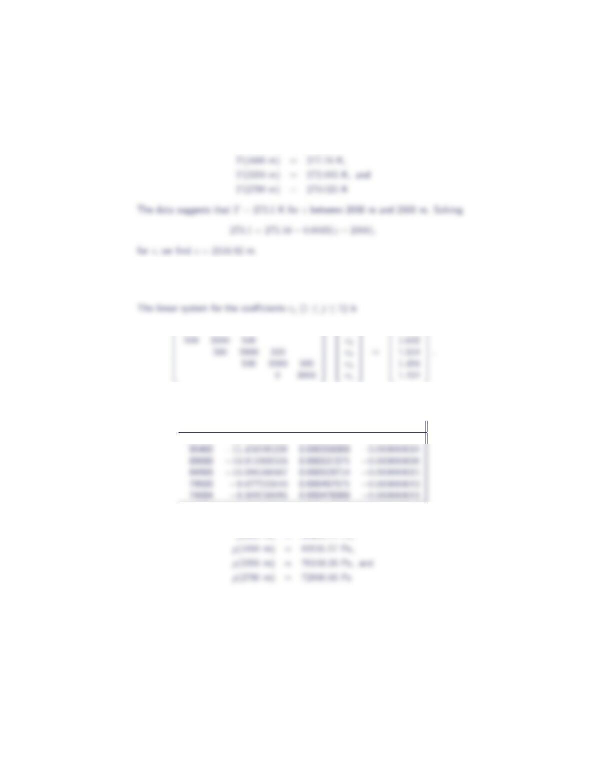
3000 0
c1
1.674
We solve this system and then use the equations (1) – (4) to determine c0,c6, the
djand the bj, respectively. The complete set of spline coefficients is
ajbjcjdj
101350 −12.027809524 0.000584429 −0.000000018
Using the appropriate piece of the cubic spline, we tind
p(800 m) = 92092.77 Pa,
3. Using the not-a-knot cubic spline interpolant, estimate the density of the stan-
dard atmosphere at an altitude of z= 800 m, 1600 m, 2350 m and 2790 m? At
what altitude is the density of the standard atmosphere 1.1000 kg/m3?
Cubic Spline Interpolation 3
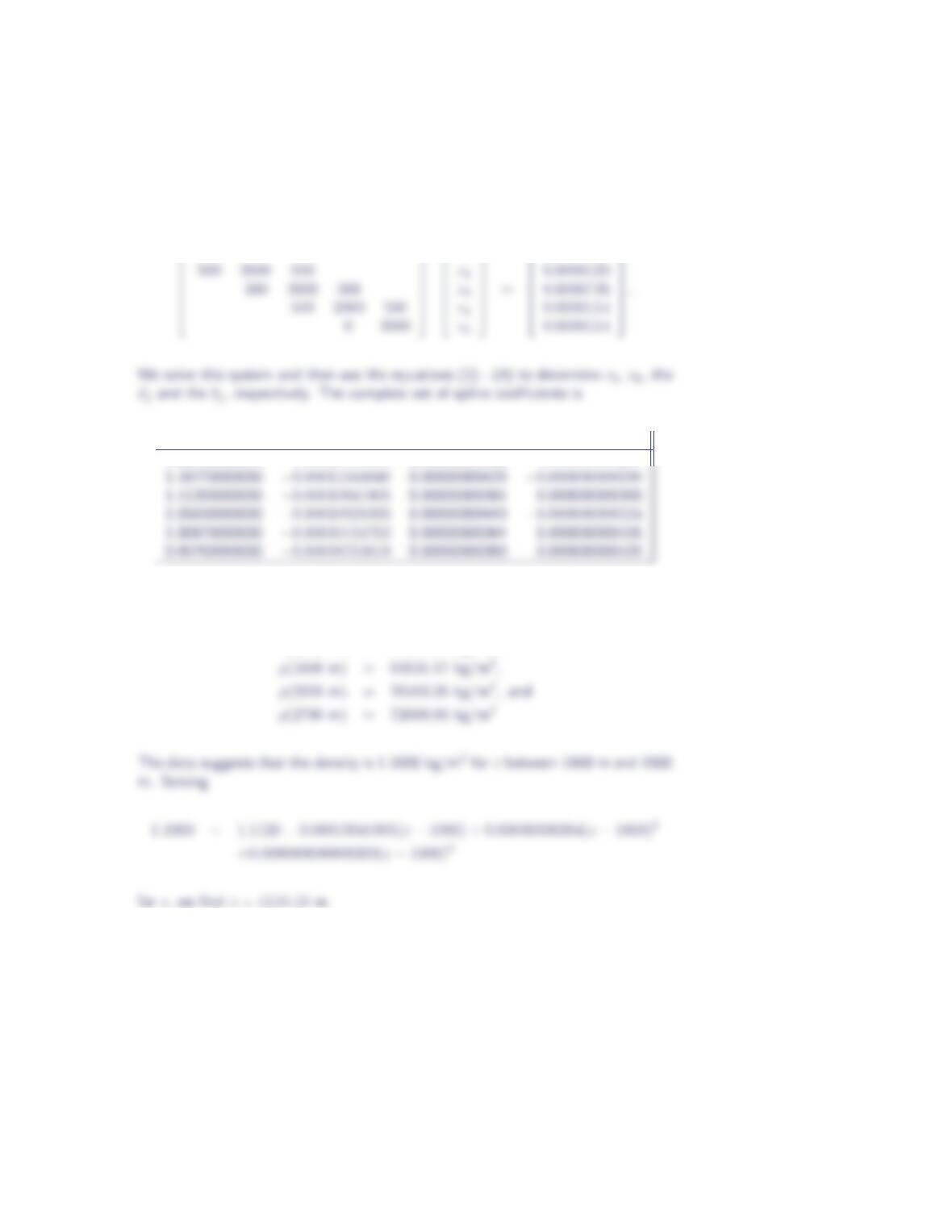
The linear system for the coefficients cj(1≤j≤5) is
3000 0
c1
0.0000126
ajbjcjdj
1.22550000000 −0.00011781905 0.00000000456 −0.000000000238
Using the appropriate piece of the cubic spline, we tind
ρ(800 m) = 92092.77 kg/m3,
Exercises 4 through 9 are based on the following data for the density, ρ, viscosity,
µ, kinematic viscosity, ν, surface tension, Υ, vapor pressure, pv, and sound
speed, a, of water as a function of temperature. This data was drawn from
Tables A.1 and A.5 in Frank White, Fluid Mechanics:
4Section 5.6
Tρ µ ν Υpva
(◦C) (kg/m3) (×10−3N·s/m2) (×10−5m2/s) (N/m) (kPa) (m/s)
0 1000 1.788 1.788 0.0756 0.611 1402
10 1000 1.307 1.307 0.0742 1.227 1447
20 998 1.003 1.005 0.0728 2.337 1482
4. Using the not-a-knot cubic spline interpolant, estimate the density of water when
T = 34◦C, 68◦C, 86◦C and 91◦C?
The complete set of spline coefficients is
ajbjcjdj
1000.0 −0.15716740304 −0.01000000000 0.00057167403
996.0 −0.30017182131 −0.01860088365 0.00086180658
988.0 −0.44523809524 −0.01041237113 0.00049361807
978.0 −0.53316151203 −0.00717231222 0.00004884634
Using the appropriate piece of the cubic spline, we tind
5. Using the not-a-knot cubic spline interpolant, estimate the viscosity of water
when
T = 34◦C, 68◦C, 86◦C and 91◦C? At what temperature is the viscosity 1.000 ×
10−3N·s/m2?
The complete set of spline coefficients is
Cubic Spline Interpolation 5
ajbjcjdj
1.788 −0.059859545287 0.001321431793 −0.000014547726
1.003 −0.024459545287 0.000448568207 −0.000004261368
0.657 −0.012274088733 0.000128523104 0.000000888577
0.467 −0.006977696981 0.000090755247 −0.000001298555
Using the appropriate piece of the cubic spline, we tind
µ(34◦C) = 0.736655 ×10⁻³N·s/m2,
6. Using the not-a-knot cubic spline interpolant, estimate the kinematic viscosity
of water when T = 34◦C, 68◦C, 86◦C and 91◦C? At what temperature is the
kinematic viscosity 1.000 ×10⁻⁵m2/s?
The complete set of spline coefficients is
ajbjcjdj
1.307 −0.037619503252 0.000895000000 −0.000015304967
0.802 −0.016636522766 0.000331596097 −0.000006794382
0.555 −0.009291815476 0.000147345361 −0.000001816381
0.414 −0.005448893900 0.000051238954 0.000000365044
Using the appropriate piece of the cubic spline, we tind
6Section 5.6
7. Using the not-a-knot cubic spline interpolant, estimate the surface tension of
water when T = 34◦C, 68◦C, 86◦C and 91◦C? At what temperature is the
surface tension 0.0650 N/m?
The complete set of spline coefficients is
ajbjcjdj
0.0756 −0.000151130032 0.000001669505 −0.000000055650
0.0728 −0.000151130032 −0.000001669505 0.000000078251
0.0696 −0.000164690415 −0.000001042572 0.000000051161
0.0662 −0.000174535776 −0.000000926500 0.000000038008
Using the appropriate piece of the cubic spline, we tind
Υ(34◦C) = 0.0705630 N/m,
8. Using the not-a-knot cubic spline interpolant, estimate the vapor pressure of
water when T = 34◦C, 68◦C, 86◦C and 91◦C?
The complete set of spline coefficients is
Cubic Spline Interpolation 7
ajbjcjdj
1.227 0.081707066151 0.002470000000 0.000045929338
4.242 0.243249463058 0.005988479381 0.000101657431
12.34 0.612085416667 0.012818711340 0.000177274699
31.16 1.347346370275 0.024433479381 0.000273188359
70.11 2.665763767182 0.042150000000 0.000317362328
Using the appropriate piece of the cubic spline, we tind
9. Using the not-a-knot cubic spline interpolant, estimate the sound speed of water
when T = 34◦C, 68◦C, 86◦C and 91◦C?
ajbjcjdj
1402.0 5.06969501718 −0.06045425258 0.00034847509
1482.0 3.06969501718 −0.03954574742 0.00025762457
1529.0 1.60603522337 −0.04318621134 0.00125826890
1551.0 0.51479810997 −0.05506121134 0.00235814003
1550.0 −0.62556915808 −0.01500000000 0.00075569158
Using the appropriate piece of the cubic spline, we tind
a(34◦C) = 1517.890943 m/s,
10. Consider the following data set
x0.0 0.5 1.0 1.5 2.0
y0.500000 1.425639 2.640859 4.009155 5.305472
y′1.500000 2.305472
(a) Construct the not-a-knot cubic spline for this data set.
(b) Construct the clamped cubic spline for this data set.
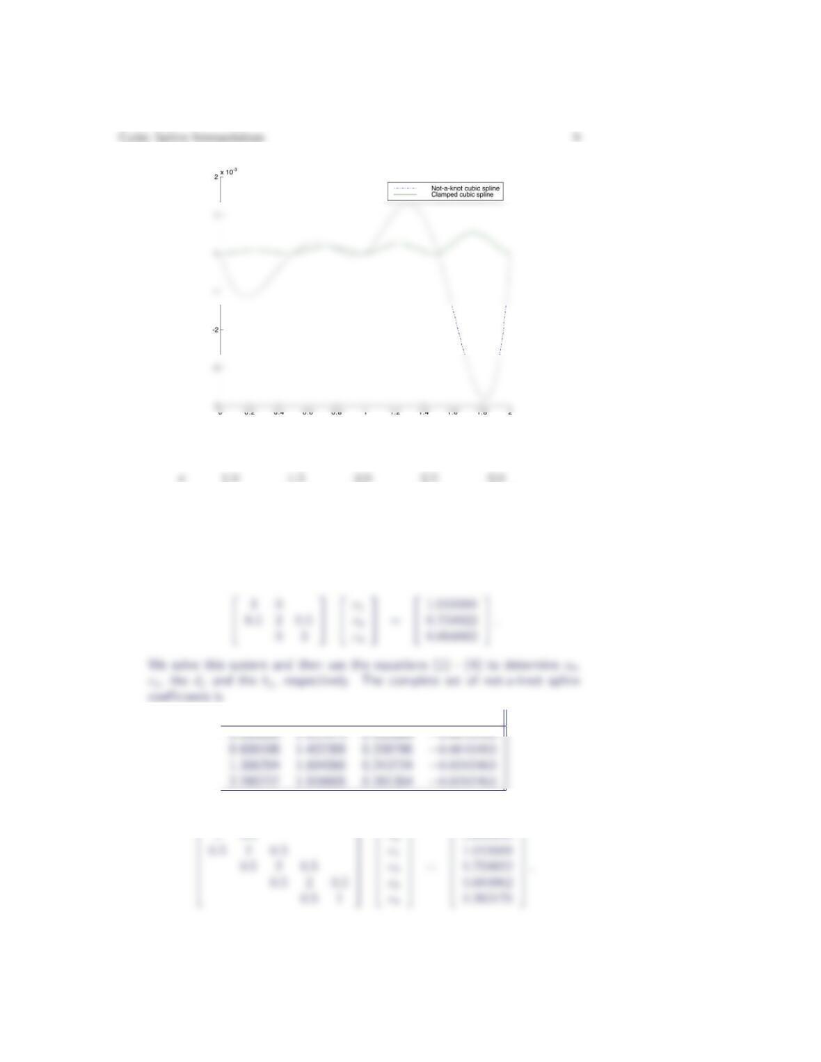
(c) The data for this problem is taken from the function y= (x+ 1)2−0.5ex.
Plot the error in each of the splines from parts (a) and (b) as a function of
x. Which spline produced the better results?
(a) The linear system for the coefficients cj(1≤j≤3) is
3 0
c1
1.737486
ajbjcjdj
0.500000 1.4854520 0.807897 −0.15249
(b) The linear system for the coefficients cj(0≤j≤4) is
1 0.5
c0
1.053834
ajbjcjdj
11. Repeat Exercise 10 for the data set
y0.000000 0.608198 1.386294 2.290727 3.295837
y′1.000000 2.098612
which is taken from the function f(x) = xln x.
(a) The linear system for the coefficients cj(1≤j≤3) is
ajbjcjdj
(b) The linear system for the coefficients cj(0≤j≤4) is
10 Section 5.6
ajbjcjdj
0.000000 1.000000 0.486076 −0.106567
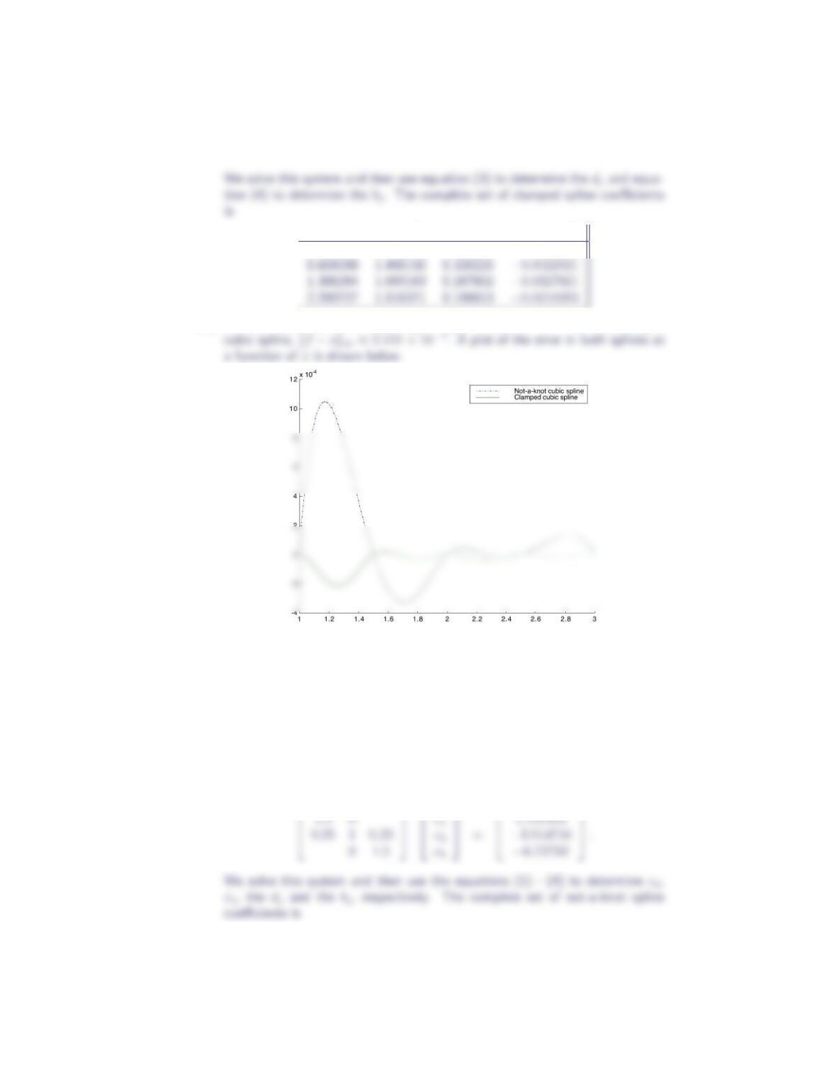
(c) For the not-a-knot cubic spline, kf−sk∞≈1.048 ×10⁻³; for the clamped
12. Repeat Exercise 10 for the data set
x0.00 0.25 0.50 0.75 1.00
y0.000000 0.176777 0.500000 0.530330 0.000000
y′0.000000 −3.141593
which is taken from the function f(x) = xsin(πx).
(a) The linear system for the coefficients cj(1≤j≤3) is
Cubic Spline Interpolation 11
ajbjcjdj
0.176777 1.321488 1.171568 −5.143808
(b) The linear system for the coefficients cj(0≤j≤4) is
0.25 1 0.25
0.25 1 0.25
c1
c3
=
1.757352
−6.727920
.
ajbjcjdj
0.176777 1.253054 1.539140 −5.519157
0.530330 −0.961547 −5.197090 2.231995
13. Experimentally determined values for the partial pressure of water vapor, pA,
as a function of distance, y, from the surface of a pan of water are given below.
The derivative of the partial pressure with respect to distance is estimated to
12 Section 5.6
be −0.0455 atm/mm when y= 0 and 0 atm/mm when y= 5. Estimate the
partial pressure at distances of 0.5 mm, 2.1 mm and 3.7 mm from the surface
of the water using a clamped cubic spline.
y(mm) 0 1 2 3 4 5
pA(atm) 0.100 0.065 0.042 0.029 0.022 0.020
2 1
1 4 1
c0
c3
=
0.0315
0.0180
.
ajbjcjdj
0.065 −0.0276986 0.00410287 0.000595694
0.029 −0.00947847 0.00233732 0.000141148
Natural Boundary Conditions:
Another set of boundary conditions which can be used when no other in-
formation is available about fis the natural (or free) boundary conditions
s′′ (a) = s′′ (b) = 0. Since s′′ (a) = s′′
0(a) = c0and s′′ (b) = s′′
n(b) = cn, the
natural boundary conditions immediately translate to
c0= 0 and cn= 0.
Combining these two equations with equation (5) for j= 1, 2, 3, …, n−1
provides a complete linear system for determining the cj. The coefficient ma-
trix for this system is tridiagonal and strictly diagonally dominant. If f′′ (a) =
f′′ (b) = 0, the natural cubic spline has a fourth-order error bound (see Birkhoff
and de Boor [7]); otherwise, the natural cubic spline produces errors that are
Cubic Spline Interpolation 13
only second-order near the boundaries (see de Boor [2]). Exercises 14 – 19 deal
with the natural cubic spline.
14. Determine the natural cubic spline for the data in the example “A Clamped
Cubic Spline.” Compare the error in the natural cubic spline to that of the
not-a-knot cubic spline.
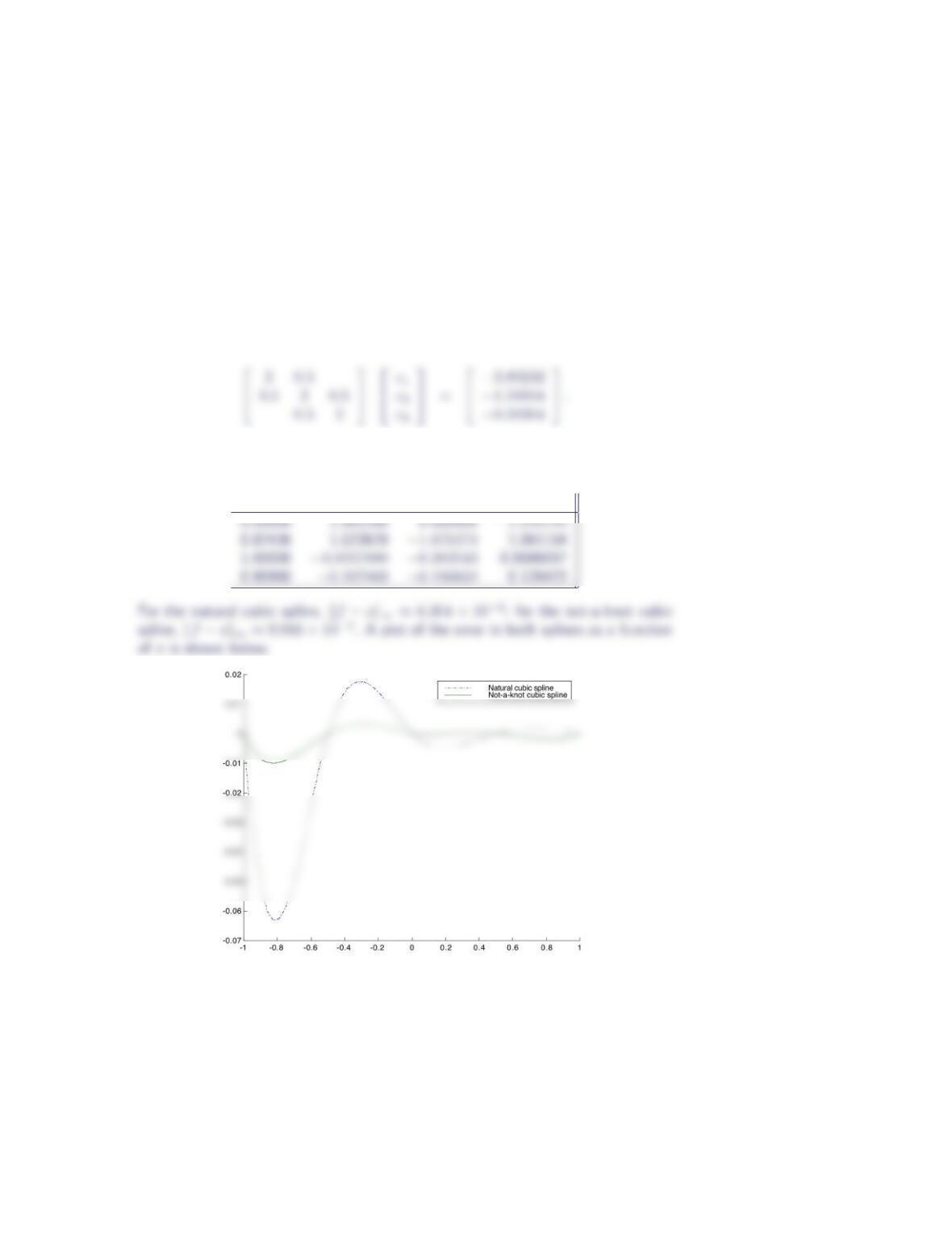
The linear system for the coefficients cj(1≤j≤3) is
We solve this system and then use equation (3) to determine the djand equation
(4) to determine the bj. The complete set of natural spline coefficients is
ajbjcjdj
15. Determine the natural cubic spline for the data in Exercise 10. Compare the
error in the natural cubic spline to that of the not-a-knot cubic spline.
14 Section 5.6
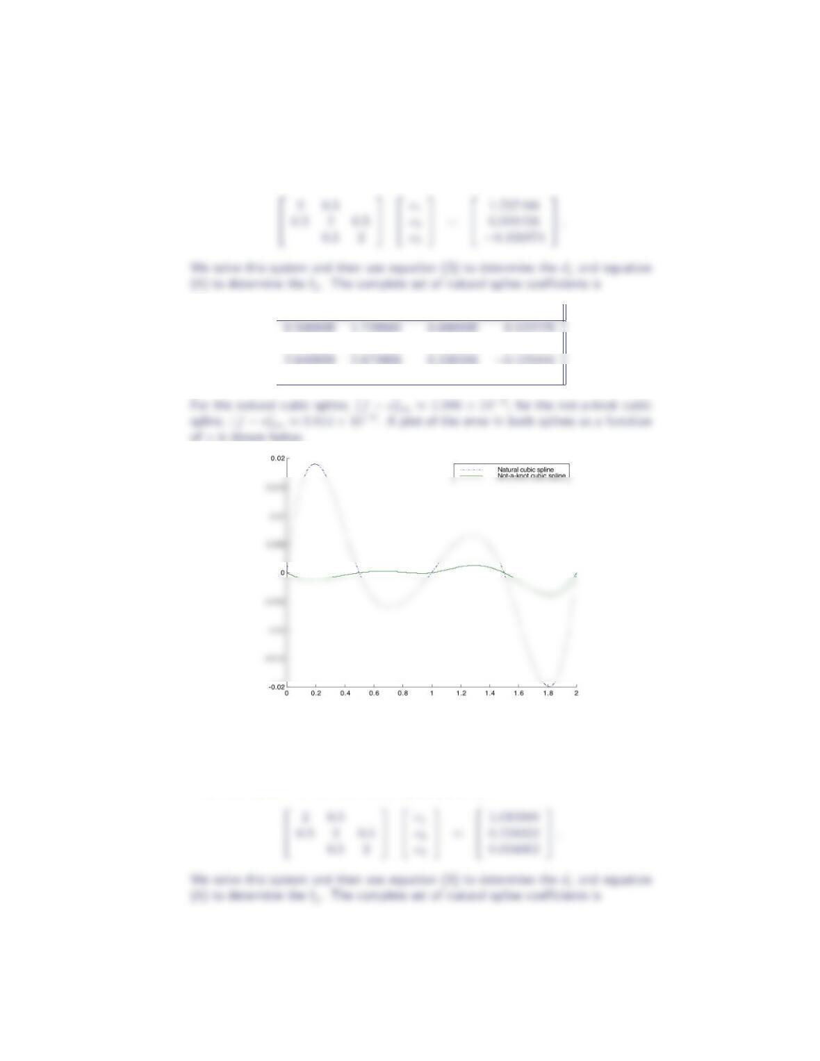
The linear system for the coefficients cj(1≤j≤3) is
ajbjcjdj
1.425639 2.112666 0.784164 −0.297232
4.009155 2.692806 −0.300516 0.200344
16. Determine the natural cubic spline for the data in Exercise 11. Compare the
error in the natural cubic spline to that of the not-a-knot cubic spline.
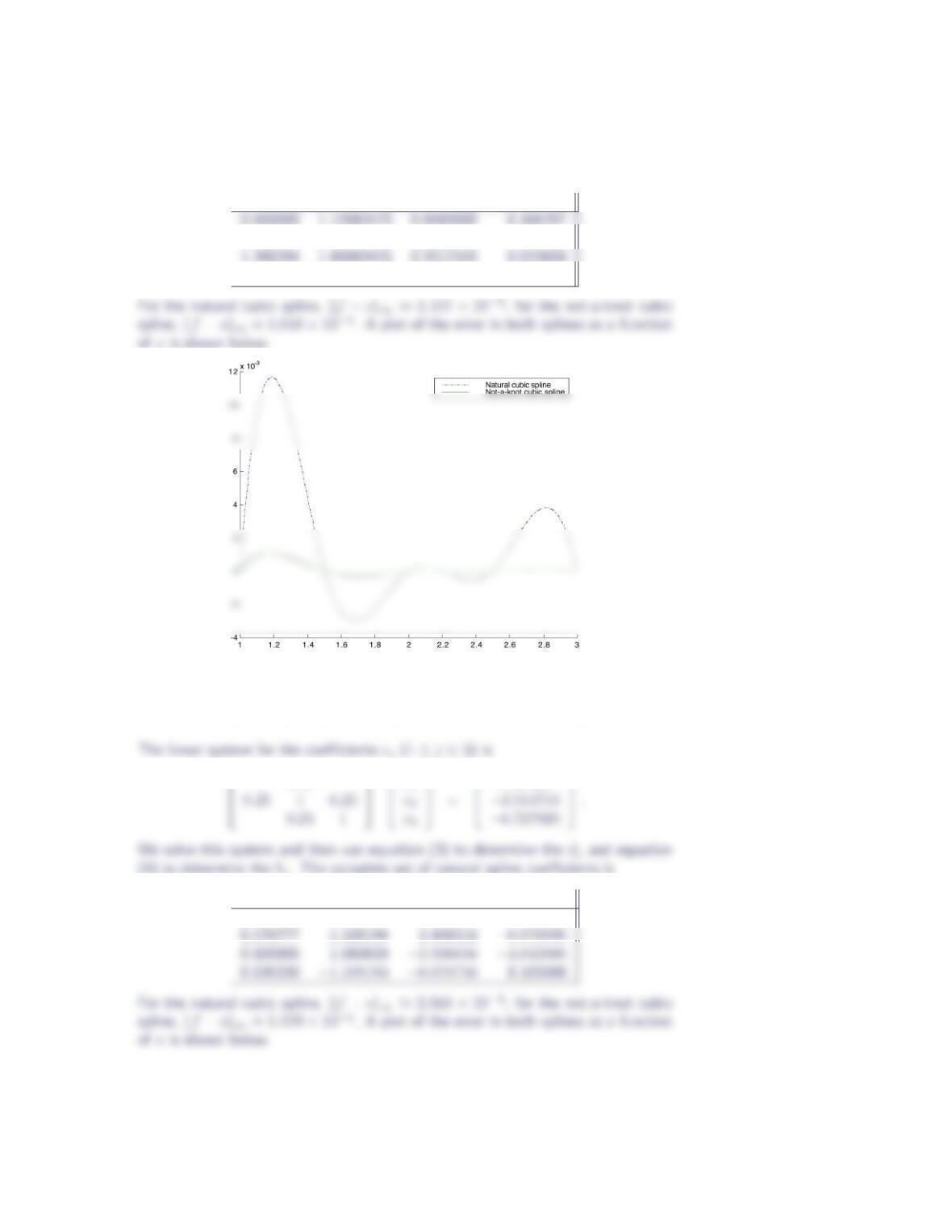
The linear system for the coefficients cj(1≤j≤3) is
Cubic Spline Interpolation 15
ajbjcjdj
0.608198 1.36952450 0.4593855 −0.172101
2.290727 1.92631250 0.2517225 −0.167815
17. Determine the natural cubic spline for the data in Exercise 12. Compare the
error in the natural cubic spline to that of the not-a-knot cubic spline.
1 0.25
c1
1.757352
(4) to determine the bj. The complete set of natural spline coefficients is
ajbjcjdj
0.000000 0.506565 0.000000 3.208688
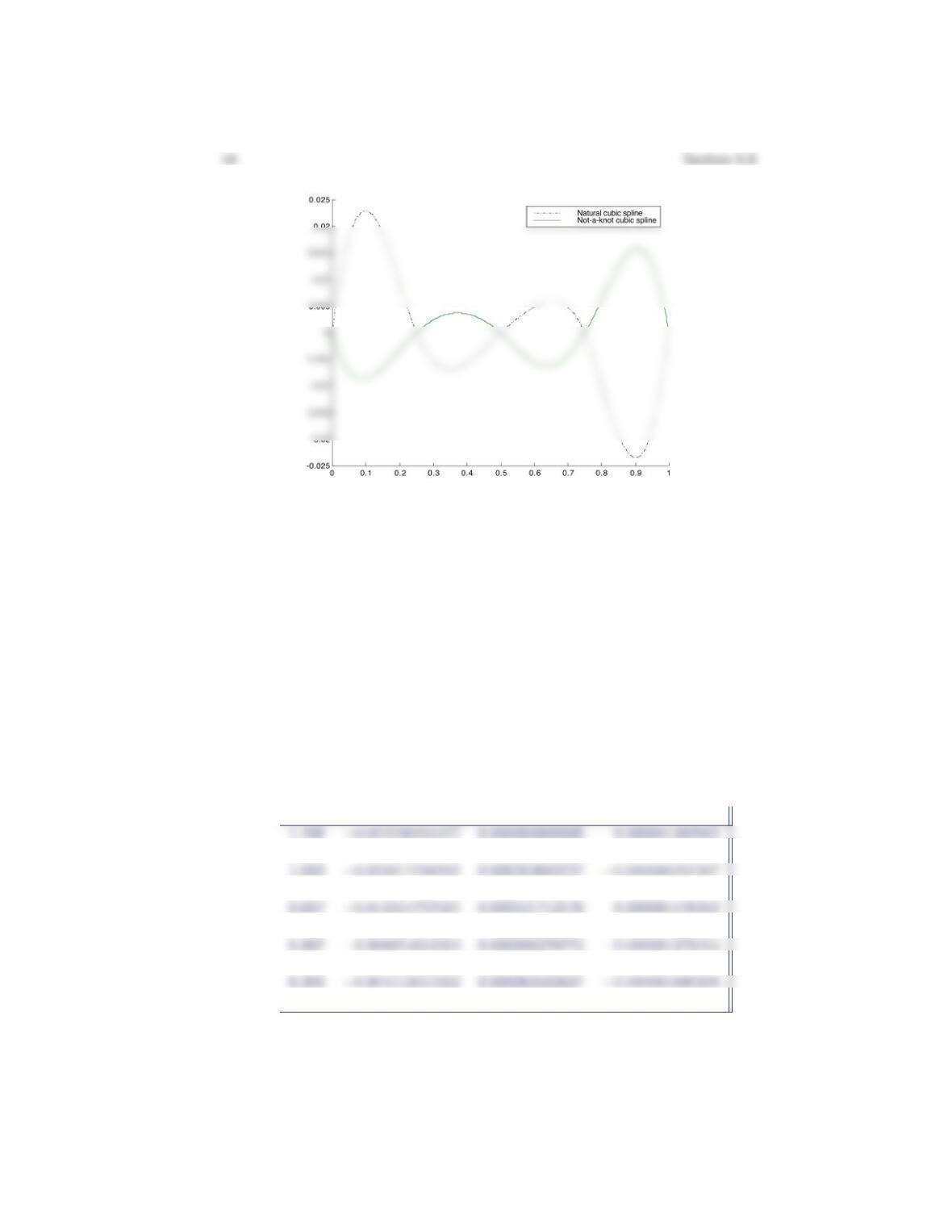
18. Determine the natural cubic spline for the following data sets. In each case,
compare the natural cubic spline with the not-a-knot cubic spline.
(a) viscosity of water (Exercise 5)
(b) vapor pressure of water (Exercise 8)
(c) sound speed of water (Exercise 9)
(d) pressure of the standard atmosphere (Exercise 2)
(e) density of the standard atmosphere (Exercise 3)
(a) The complete set of natural spline coefficients is
ajbjcjdj
1.307 −0.039839489545 0.001239076568 −0.000029512761
0.799 −0.016913364086 0.000346148524 −0.000007481212
0.548 −0.009447607656 0.000157002762 −0.000002224200
0.405 −0.005553143091 0.000051890150 0.000000342416
0.316 −0.003496395622 0.000029459343 −0.000000981978
(b) The complete set of natural spline coefficients is
Cubic Spline Interpolation 17
ajbjcjdj
0.611 0.052390086309 0.000000000000 0.000092099137
2.337 0.145330604166 0.003768103571 0.000074883601
7.375 0.393438372016 0.009013449999 0.000129271280
19.92 0.920106604060 0.017870196410 0.000251914318
47.35 1.896554084829 0.028919299744 0.000902529177
70.11 2.745698832906 0.055995175064 −0.001866505835
(c) The complete set of natural spline coefficients is
ajbjcjdj
1447.0 4.05867588358 −0.06619861746 0.00103310291
1509.0 2.36278648656 −0.03297926194 −0.00032993867
1542.0 1.12033492823 −0.00551104972 −0.00165224431
1553.0 0.12190250866 0.01582456581 −0.00180148167
1550.0 −0.61369980703 −0.01294502895 0.00043150096
(d) The complete set of natural spline coefficients is
ajbjcjdj
101350.0 −11.859197436 0.00000000000 0.00000047679
89889.0 −10.900382051 0.00048726154 0.00000003501
74684.0 −9.354528205 0.00060158462 −0.00000040106
(e) The complete set of natural spline coefficients is
ajbjcjdj
1.1677 −0.00011379128 0.00000000543 −0.00000000000129
1.0583 −0.00010528667 0.00000000459 −0.00000000000084
0.9570 −0.00009722205 0.00000000487 −0.00000000000324
19. Show that the natural cubic spline satisties the following minimum curvature
property: Let gbe any function, continuous and twice continuously differen-
18 Section 5.6
tiable on the interval [a, b], which interpolates fover the partition
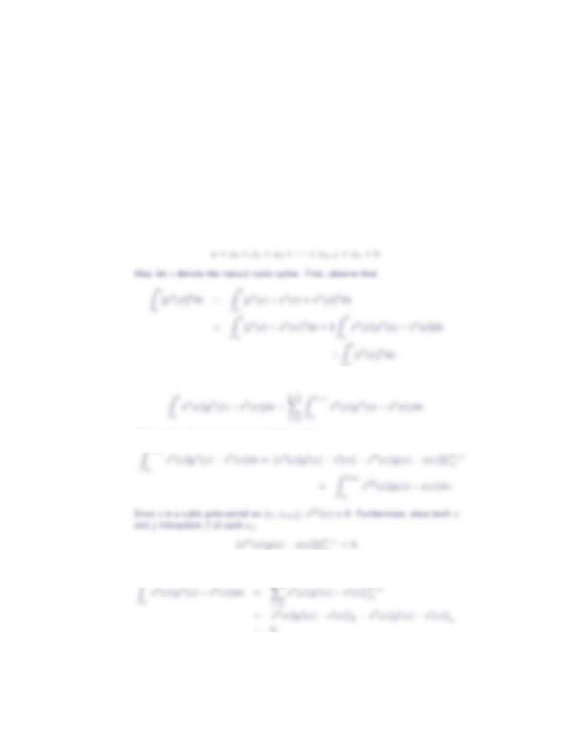
a=x0< x1< x2<···< xn−1< xn=b.
Then
Zb
a
[s′′ (x)]2dx ≤Zb
a
[g′′ (x)]2dx,
where sis the natural cubic spline.
Let gbe any function, continuous and twice continuously differentiable on the
interval [a, b], which interpolates fover the partition
Next, focus on the term
After integrating by parts twice, it follows that
Zxi+1
xi= 0.
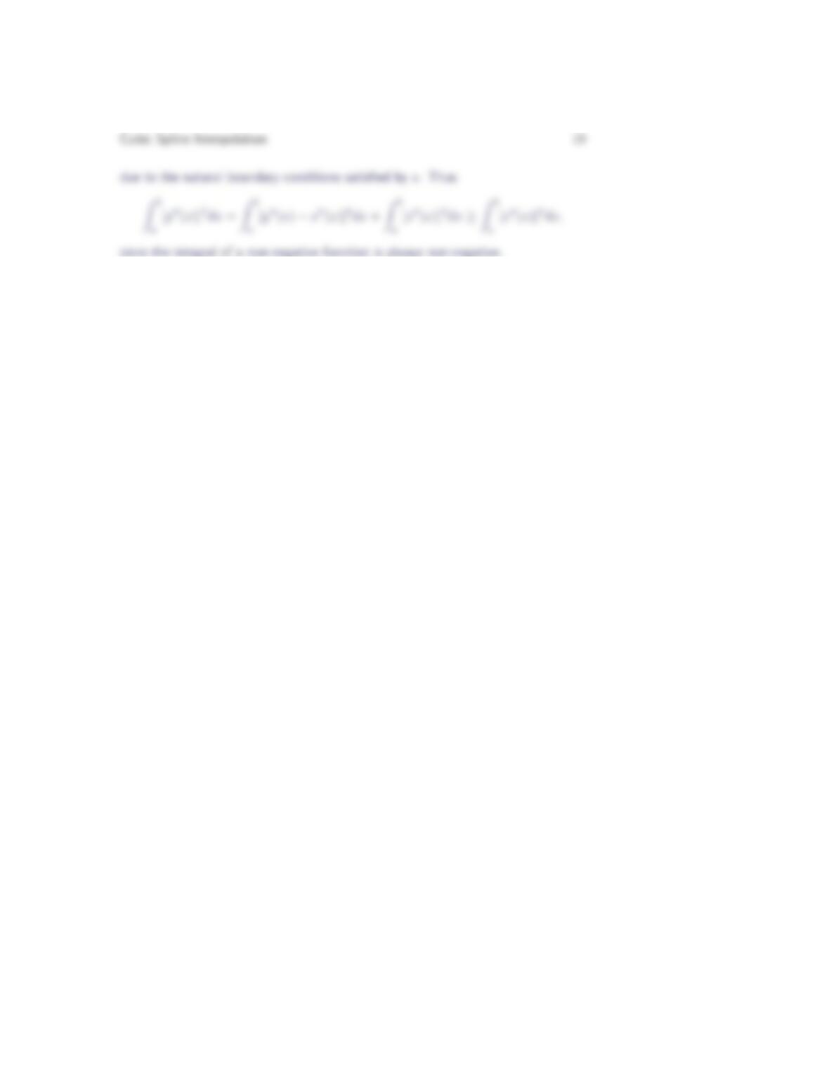
Therefore,
Zb
n−1
X