1
CHAPTER 5
Problem 5.1
In Section 5.2 we developed recurrence formulas for
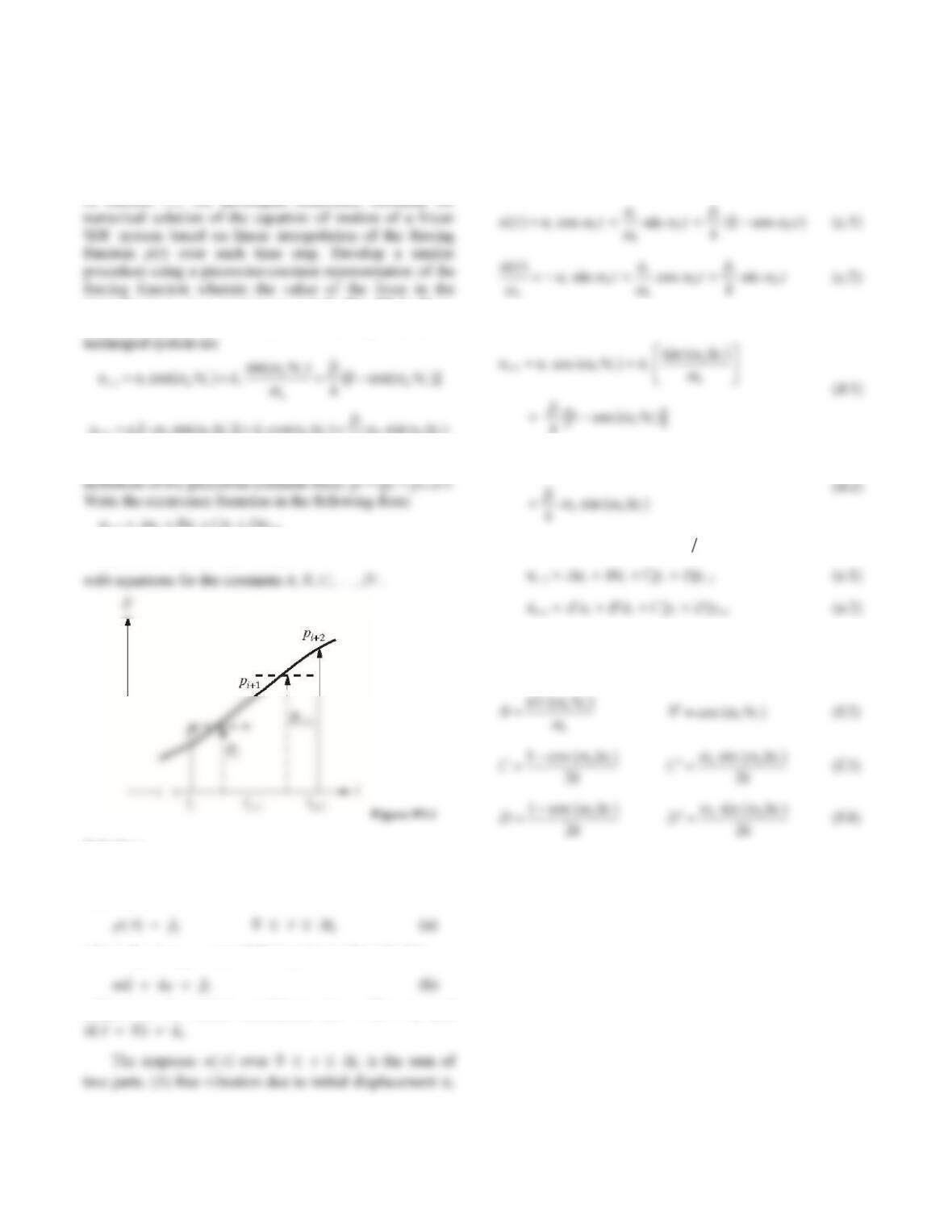
interval ti to ti+1 is a constant equal to ᷉᷉pi (Fig. P5.1). Show
that the recurrence formulas for the response of an
1[sin()]cos() sin()
iinnii ni nni
uu tu t t
k
Specialize the recurrence formulas for the following
11iiiii
uAuBuCpDp
11iiiii
uAuBuCpDp
Solution:
Over the time interval ttt
ii
1 the excitation
function is
where tt t
ii i
1 and the equation to be solved is
subject to the initial conditions uu
i
()
0 and
and velocity
ui at
0; and (2) response to step force
pi
with zero initial conditions:
Evaluate Eqs. (c) at
ti or tt t
ii
:
k
1sin ( ) cos ( )
iin ni i ni
uu tu t
Substituting
()ppp
iii
12 gives
where
cos ( )
ni
A
t
sin ( )
nni
A
t
(f.1)
2
Problem 5.2
Solve Example 5.1 using the piecewise-constant approxi-
Solution:
1. Initial calculations.
3.6932 0.8090 0.1847 0.1847ABCD
2. Apply the recurrence Eqs. (e) of Problem 5.1.
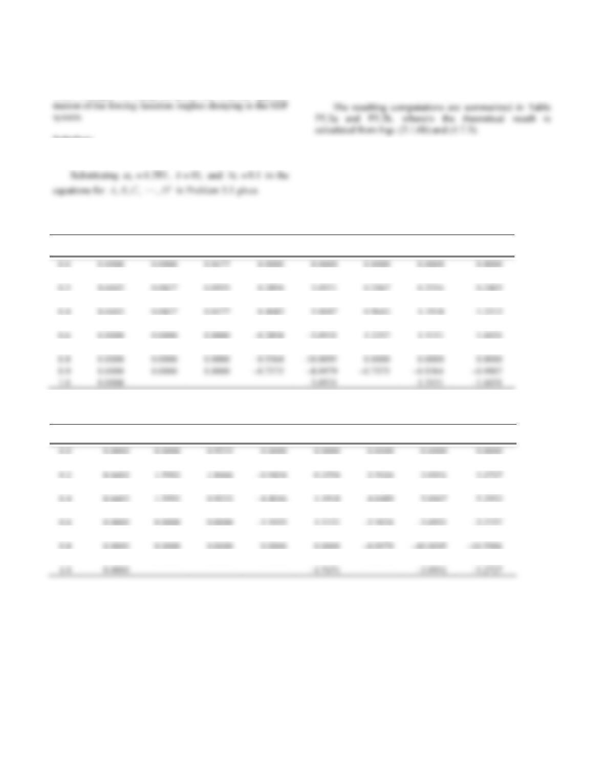
Table P5.2a: Numerical solution using piecewise constant interpolation of excitation
ti i
p Cpi
D
p
i1 Bui
ui
A
ui ui Theoretical ui
0.1 5.0000 0.0477 0.0827 0.0864 0.9233 0.0386 0.0477 0.0333
0.3 10.0000 0.0955 0.0827 0.4682 5.0047 0.5454 0.6742 0.6789
0.5 5.0000 0.0477 0.0000 0.2030 2.1698 1.2644 1.5628 1.6364
0.7 0.0000 0.0000 0.0000 –0.7575 –8.0978 0.7575 0.9364 0.9907
Table P5.2b: Numerical solution using piecewise constant interpolation of excitation
ti
p
i
Cp
i
Dp
i1
Au
i ui
Bu
i
ui Theoretical
ui
0.1 5.0000 0.9233 1.5992 –0.1763 0.0477 0.7470 0.9233 0.9769
0.3 10.0000 1.8466 1.5992 –2.4899 0.6742 4.0489 5.0047 5.2953
0.5 5.0000 0.9233 0.0000 –5.7718 1.5628 1.7554 2.1698 2.2958
0.7 0.0000 0.0000 0.0000 –3.4582 0.9364 –6.5513 –8.0978 –8.5680
0.9 0.0000 0.0000 0.0000 3.4582 –0.9364 –6.5513 –8.0979 –8.5680
3
Problem 5.3
Solve the problem in Example 5.1 by the central difference
method, implemented by a computer program in a
language of your choice, using ∆t = 0.1 sec. Note that this
problem was solved as Example 5.2 and that the results
were presented in Table E5.2.
Solution:
Problem 5.4
Repeat Problem 5.3 using ∆t = 0.05 sec. How does the time
step affect the accuracy of the solution?
Solution:
1.0 Initial calculations.
0.2533 10 0.1592
mkc
p
1.3 () .kmt ct
1.4 amt ct() .
1.5 bk mt 2 192 64
() .
2.0 Calculation for each time step.
2.1 11
ˆ99.73 192.64
ii i ii i i
p p au bu p u u
3.0 Repetition for next time step.
theoretical result is also included.
Comparison with Problem 5.3 and theoretical solution:
Table P5.4b shows this comparison, where the smaller
t is seen to give more accurate results.
Table P5.4b
ti ut
i(.)
01 ut
i(.)005
ui
(Theoretical)
0.10 0.0000 0.0251 0.0328
0.30 0.6293 0.6442 0.6487
0.60 1.5412 1.4955 1.4814
0.90 –0.8968 –0.8038 –0.7751
Table P5.4a: Numerical solution by central difference method
ti
p
i ui1 ui
pi [Eq. (2.1)] ui1 [Eq. (2.2)] Theoretical ui1
0.00 0.0000 0.0000 0.0000 0.0000 0.0000 0.0042
0.10 5.0000 0.0000 0.0251 9.8448 0.0957 0.1053
0.20 8.6602 0.0957 0.2234 42.1576 0.4096 0.4176
0.30 10.0000 0.4096 0.6442 93.2417 0.9060 0.9060
0.40 8.6603 0.9060 1.1656 142.8465 1.3880 1.3782
0.50 5.0000 1.3880 1.5374 162.7449 1.5814 1.5665
0.60 0.0000 1.5814 1.4955 130.3811 1.2669 1.2602
0.70 0.0000 1.2669 0.9223 51.3267 0.4987 0.5101
0.80 0.0000 0.4987 0.0398 –42.0695 –0.4088 –0.3832
0.90 0.0000 –0.4088 –0.8038 –114.0761 –1.1085 –1.0802
1.00 0.0000 –1.1085 –1.2960 –139.1210 –1.3518 –1.3349
5
Problem 5.5
Example 5.1, but the damping ratio is ζ = 20%. Determine
the response of this system to the excitation of Example
5.1 by the central difference method using ∆t = 0.05 sec.
Plot the response as a function of time, compare with the
Solution:
1.0 Initial calculations.
m
k
c0 2533 10 0 6366..
1.1
()u
p
cu ku m
0000 0
2.0 Calculations for each time step.
p
uu
ii i
94 95 192 64
1
..
3.0 Repetition for the next time step.
Computational steps 2.1 and 2.2 are repeated for i = 0,
1, 2, 3, … leading to Table P5.5; also included is the
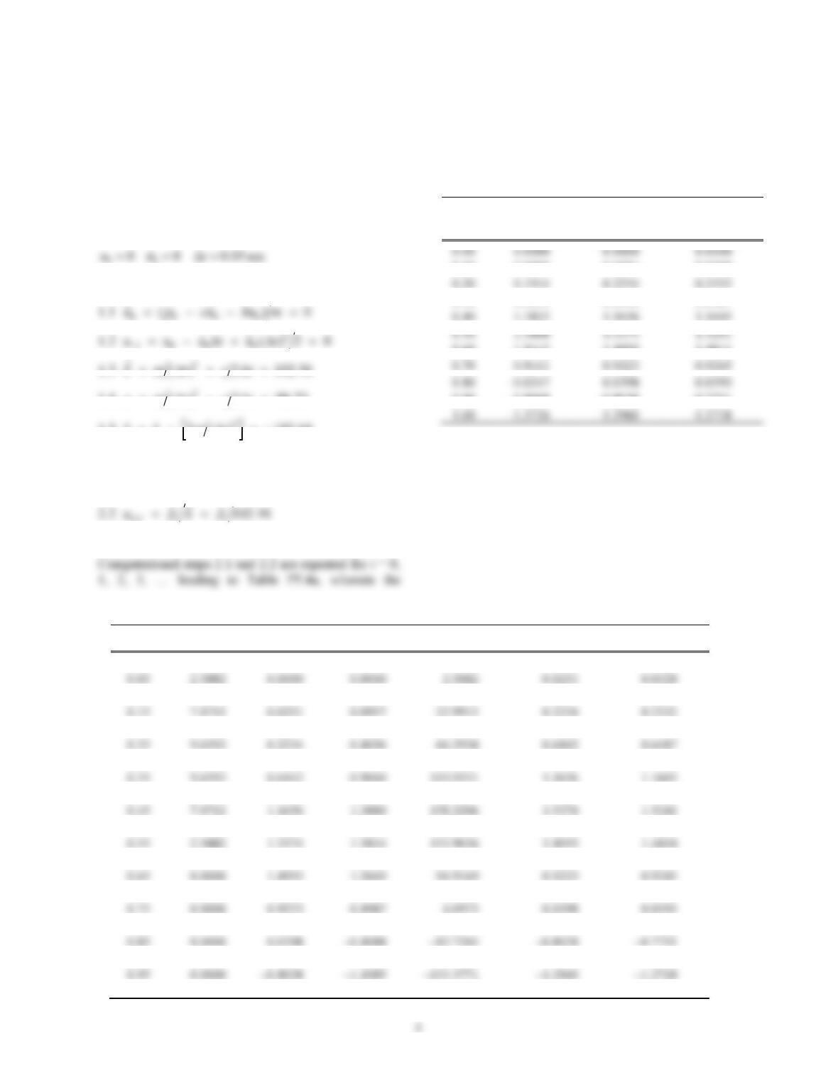
The response of systems with
005. and
020.
is compared in the accompanying figure; numerical
solution gives the peak displacement in.5814.1
0
u for
2
Time (sec)
0.20 (Problem 5.5)
Table P5.5: Numerical solution by central difference method
ti
p
i ui1 ui
p
i [Eq. (2.1)] ui1 [Eq. (2.2)] Theoretical ui1
0.05 2.5882 0.0000 0.0000 2.5882 0.0240 0.0313
0.15 7.0711 0.0240 0.0894 22.0161 0.2044 0.2133
0.25 9.6593 0.2044 0.3673 61.0036 0.5665 0.5704
0.35 9.6593 0.5665 0.7824 106.5884 0.9898 0.9854
0.45 7.0711 0.9898 1.1612 136.7796 1.2702 1.2593
0.55 2.5882 1.2702 1.2947 131.3981 1.2202 1.2087
0.65 0.0000 1.2202 1.0412 84.7074 0.7866 0.7888
0.75 0.0000 0.7866 0.4891 19.5312 0.1814 0.1957
0.85 0.0000 0.1814 –0.1068 –37.8014 –0.3510 –0.3316
0.95 0.0000 –0.3510 –0.5338 –69.4929 –0.6453 –0.6298
6
Problem 5.6
Solve the problem in Example 5.1 by the central difference
method using ∆t = 1/3 sec. Carry out your solution to 2 sec,
and comment on what happens to the solution and why.
Solution:
1.0 Initial calculations.
m
k
c0 2533 10 0 1592..
1.5
bk mt 2 5 441
2
() .
2.0 Calculations for each time step.
2.1
p p au bu
ii i i
1
2.2
upkp
ii i
12 518
.
3.0 Repetition for the next time step.
Computational steps 2.1 and 2.2 are repeated for i = 0,
Table P5.6: Numerical solution by central difference method
ti
p
i ui1 ui
p
i [Eq. (2.1)] ui1 [Eq. (2.2)] Theoretical ui1
33.0 9.8481 0.0000 0.0000 9.8481 3.9104 1.1595
1.00 0.0000 3.9104 –8.4474 37.9773 15.0796 0.1998
166. 0.0000 15.0796 –25.7299 109.2072 43.3626 –0.9262
p
7
Problem 5.7
Solve the problem in Example 5.1 by the constant average
acceleration method, implemented by a computer program
in a language of your choice, using ∆t = 0.1 sec. Note that
this problem was solved as Example 5.3, and the results are
presented in Table E5.3. Compare these results with those
of Example 5.2, and comment on the relative accuracy of
the constant average acceleration and central difference
methods.
Solution:
The solution to this problem is available as Example 5.3 in
Table P5.7
i
t
)5.3Ex.(
i
u
(ave. accel.)
)5.2Ex.(
i
u
(cent. diff.)
i
u
(Theoretical)
0.00 0.0000 0.0000 0.0000
0.20 0.2326 0.1914 0.2332
0.40 1.0825 1.1825 1.1605
0.60 1.4230 1.5412 1.4814
0.80 0.1908 –0.0247 0.0593
8
Problem 5.8
Repeat Problem 5.7 using ∆t = 0.05 sec. How does the time
step affect the accuracy of the solution?
Solution:
1.0 Initial calculations.
1.1 0)( 0000 mkuucpu
1.2 sec05.0Δ t
1.3
7.411Δ2)Δ(4 2
1 ctmta
3 ma
2.0 Calculations for each time step.
2.1 iiiii uauauapp 32111
ˆ
2.3
iiii uuutu
11 )Δ2(
3.0 Repetition for the next time step.
Steps 2.1 through 2.4 are repeated for successive time steps
and are summarized in Table P5.8a, wherein the theoretical
result is also included.
Table P5.8b
i
t (0.1)
i
ut (0.05)
i
ut i
u (Theoretical)
0.00 0.0000 0.0000 0.0000
0.60 1.4230 1.4673 1.4814
0.70 0.9622 0.9360 0.9245
0.80 0.1908 0.0950 0.0593
Table P5.8a: Numerical solution by average acceleration method
i
t i
p i
p
ˆ i
u
i
u
i
u
Theoretical
i
u
0.00 0.0000 0.0000 0.0000 0.0000 0.0000 0.0000
0.10 5.0000 15.0291 17.7448 0.9347 0.0356 0.0328
0.20 8.6603 98.2134 23.0598 3.0774 0.2329 0.2332
0.30 10.0000 269.4111 11.1778 4.8944 0.6389 0.6487
0.40 8.6603 480.6894 –13.8430 4.8143 1.1400 1.1605
0.50 5.0000 632.5507 –40.7761 2.0522 1.5002 1.5241
0.60 0.0000 618.6631 –56.1012 –2.9025 1.4673 1.4814
0.70 0.0000 394.6766 –32.2874 –7.4242 0.9360 0.9245
0.80 0.0000 40.0653 1.8857 –8.9689 0.0950 0.0593
0.90 0.0000 –308.0604 33.3378 –7.1505 –0.7306 –0.7751
1.00 0.0000 –523.1134 50.7592 –2.8323 –1.2406 –1.2718
9
Problem 5.9
the solution.
Solution:
1.0 Initial calculations.
m
k
c0 2533 10 0 1592..
00 0
1.1 0)( 0000 mkuucpu
2.0 Calculations for each time step.
2.1 iiiii uauauapp 32111
ˆ
2.2 07.20
ˆ
ˆ
ˆ111 iii pkpu
11
iiii
2.4
21
4( ) 4Δ
iiiii
utuu tuu
Steps 2.1 through 2.4 are repeated for successive time steps
and are summarized in Table P5.9; also included is the
theoretical result, calculated from Eq. (3.2.5)—valid for
Table P5.9: Numerical solution by average acceleration method
i
t i
p i
p
ˆ i
u
i
u
i
u Theoretical i
u
33.0 9.8481 9.8481 17.6612 2.9435 0.4906 0.8189
1.00 0.0000 –0.7161 4.9180 –5.5842 –0.0357 –1.2718
10
Problem 5.10
Solve the problem of Example 5.1 by the linear
acceleration method, implemented by a computer program
in a language of your choice, using ∆t = 0.1 sec. Note that
this problem was solved as Example 5.4 and that the
results are presented in Table E5.4. Compare with the
solution of Example 5.3, and comment on the relative
accuracy of the constant average acceleration and linear
acceleration methods.
Solution:
The solution to this problem is available as Example
5.4 in the book. Table P5.10 compares the numerical
Table P5.10
i
t
)5.3Ex.(
i
u
(avg. accel.)
)5.4Ex.(
i
u
(lin. accel.)
i
u
(Theoretical)
0.00 0.0000 0.0000 0.0000
0.20 0.2326 0.2193 0.2332
0.40 1.0825 1.1130 1.1605
0.60 1.4230 1.4625 1.4814
0.80 0.1908 0.1273 0.0593
11
Problem 5.11
Repeat Problem 5.10 using ∆t = 0.05 sec. How does the
time step affect the accuracy of the solution?
Solution:
1.0 Initial calculations.
1.3
2
16 (Δ ) 3 Δ 617.5atmtc
2.0 Calculations for each time step.
111 2 3
ˆ
ii i i i
ppauauau
2.3
11
(3 Δ ) 2 Δ 2
iiiii
utuuutu
2.4
2
11
6(Δ) 6Δ 2
iiiii
utuutuu
3.0 Repetition for the next time step.
Steps 2.1 through 2.4 are repeated for successive time steps
and are summarized in Table P5.11a, wherein the
smaller tΔ gives more accurate results.
i
t (0.1)
i
ut (0.05)
i
ut i
u (Theoretical)
0.20 0.2326 0.2298 0.2332
0.40 1.0825 1.1484 1.1605
0.50 1.4309 1.5124 1.5241
0.60 1.4230 1.4767 1.4814
0.70 0.9622 0.9318 0.9245
Table P5.11a: Numerical solution by average acceleration method
i
t i
p i
p
ˆ i
u
i
u
i
u
Theoretical
i
u
0.05 2.5882 2.5882 9.8995 0.2475 0.0041 0.0042
0.15 7.0711 65.0086 22.5977 1.9537 0.1036 0.1053
0.25 9.6593 258.5228 19.2544 4.1586 0.4120 0.4176
0.35 9.6593 561.9174 –0.4782 5.1829 0.8955 0.9060
0.45 7.0711 856.8575 –28.3544 3.7534 1.3656 1.3782
0.55 2.5882 977.2661 –51.0841 –0.2943 1.5575 1.5665
0.65 0.0000 791.4030 –46.3047 –5.5502 1.2613 1.2602
0.75 0.0000 328.3373 –15.1958 –8.6910 0.5233 0.5101
0.85 0.0000 –227.6315 19.6325 –8.4494 –0.3628 –0.3832
0.95 0.0000 –666.6023 45.1569 –5.1169 –1.0624 –1.0802
12
Problem 5.12
Solve the problem of Example 5.5 by the central difference
method, implemented by a computer program in a
language of your choice, using ∆t = 0.05 sec.
Solution:
The governing equation is
where
and
The solution steps are summarized in Table P5.12.
Table P5.12: Numerical solution by central difference method
ti
p
i ()
f
S
i ui1 ui
pi
ui1 ui1
0.00 0.0000 0.0000 0.0000 0.0000 0.0000 0.0000 0.0000
0.10 5.0000 0.9566 0.0000 0.0251 9.8448 0.9566 0.0957
0.20 8.6602 4.0964 0.0957 0.2234 42.1576 3.1398 0.4096
0.30 10.0000 7.5000 0.4096 0.6442 93.2417 4.9638 0.9060
0.40 8.6603 7.5000 0.9060 1.1808 150.0748 5.5225 1.4583
0.50 5.0000 7.5000 1.4583 1.7230 201.2263 4.9704 1.9553
0.60 0.0000 7.5000 1.9553 2.1327 229.6683 2.7637 2.2317
0.70 0.0000 7.5000 2.2317 2.2547 226.8420 –0.2746 2.2042
0.80 0.0000 4.4905 2.2042 2.0824 195.8701 –3.0095 1.9033
13
Problem 5.13
Solve Example 5.5 by the constant average acceleration
method with Newton–Raphson iteration, implemented by a
computer program in a language of your choice. Note that
this problem was solved as Example 5.5 and the results
were presented in Table E5.5.
Solution:
14
Problem 5.14
Solve Example 5.5 by the constant average acceleration
method with Newton–Raphson iteration, implemented by a
computer program in a language of your choice. Note that
this problem was solved as Example 5.5 and the results
were presented in Table E5.5.
Solution:

15
Problem 5.15
Solve the problem of Example 5.5 by the linear accelera-
tion method with Newton–Raphson iteration using ∆t = 0.1
sec.
Solution:
Table P5.15 shows the results obtained by the linear
acceleration method with Newton–Raphson iteration.
Table P5.15: Numerical solution by linear acceleration method with Newton–Raphson iteration
i
t i
p i
R
ˆ or
j
i
R
ˆ
i
T
k or
j
i
T
k
i
T
k
ˆ or
j
i
T
k
ˆ
j
u
i
u or
1j
i
u
1j
i
S
f i
u
i
u
0.10 5.0000 5.0000 10 166.756 0.0300 0.0300 0.2998 0.8995 17.9904
0.30 10.0000 66.2473 10 166.756 0.3973 0.6166 6.1660 4.7716 12.1372
3.6300 0 156.756 0.0232 1.1362 7.5000 5.4366 1.1636
0.60 0.0000 61.0910 0 156.756 0.3897 2.0519 7.5000 2.6396 –31.2682
0.80 0.0000 –28.6900 0 156.756 –0.1830 1.9797 5.6698
0.90 0.0000 –61.7237 10 166.756 –0.3701 1.6205 2.0781 –4.2360 –5.5417
16
Problem 5.16
Solve the problem of Example 5.5 by the linear
acceleration method with modified Newton–Raphson
iteration using ∆t = 0.1 sec.
Solution:
Table P5.16 shows the results obtained by the linear
acceleration method with modified Newton–Raphson
iteration.
Observe that more iterations are necessary compared
to Problem 5.15
Table P5.16: Numerical solution by linear acceleration method with modified Newton-Raphson iteration
i
t i
p i
R
ˆ or
j
i
R
ˆ
i
T
k or
j
i
T
k
i
T
k
ˆ or
j
i
T
k
ˆ
j
u
i
u or
1j
i
u
1j
i
S
f i
u
i
u
0.00 0.0000 0.0000 0.0000 0.0000 0.0000
0.20 8.6603 31.5748 10 166.756 0.1893 0.2193 2.1933 2.9819 23.6566
0.40 8.6603 82.7769 10 166.756 0.4964 1.1130 7.5000
0.2177 1.305E-3 1.1361 7.5000
0.50 5.0000 82.4513 0 156.756 0.5260 1.6621 7.5000 4.8486 –12.9171
0.70 0.0000 17.3643 0 156.756 0.1108 2.1626 7.5000 –0.3922 –29.3627