57
CHAPTER 5
TIME SERIES AND THEIR COMPONENTS
ANSWERS TO PROBLEMS AND CASES
1. The purpose of decomposing a time series variable is to observe its various elements
in isolation. By doing so, insights into the causes of the variability of the series are
2 . The multiplicative components model works best when the variability of the time
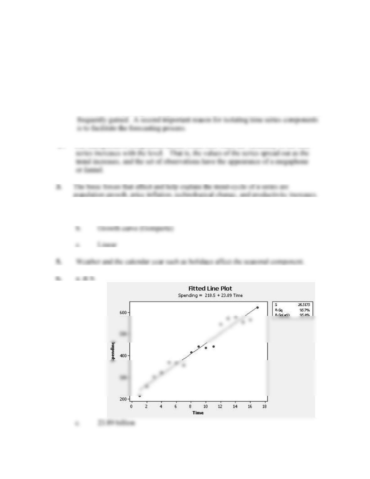
4. a. Exponential
58
7. a. & b.
12. Sales Seasonal Deseasonalized
Month ($ Thousands) Index (%) Data
59
Jan 125 51 245
Jun 241 99 243
Jul 230 96 240
13. a. & b. Would use both the trend and seasonal indices to forecast although seasonal
component is not strong in this example (see plot and seasonal indices below).
Fitted Trend Equation
Seasonal Indices
Period Index
60
1 0.969
Forecasts
c. The forecast for third quarter is a bit low compared to Value
61
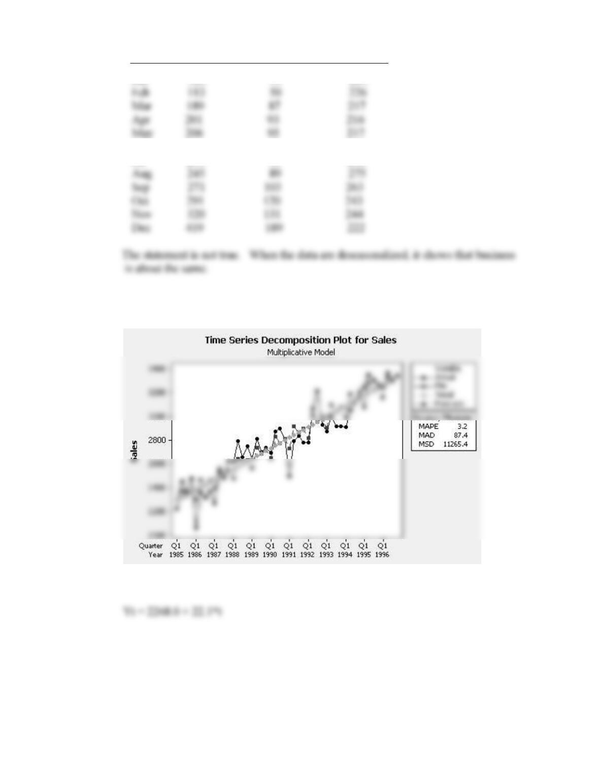
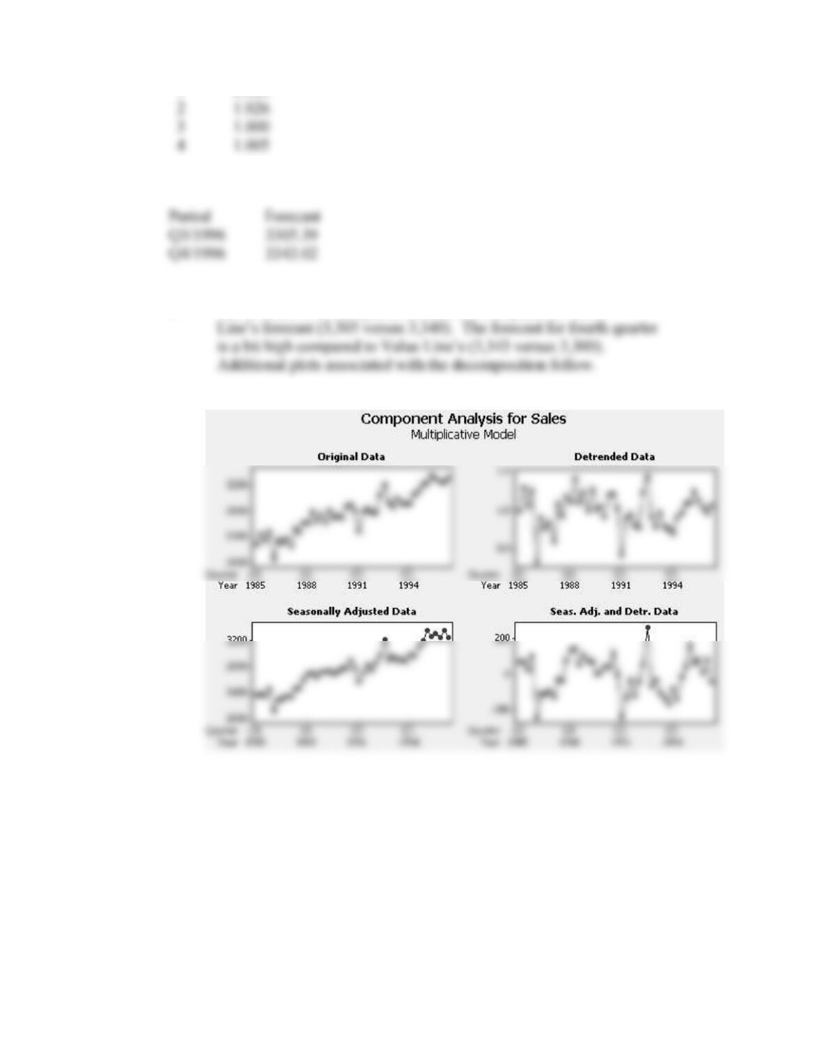
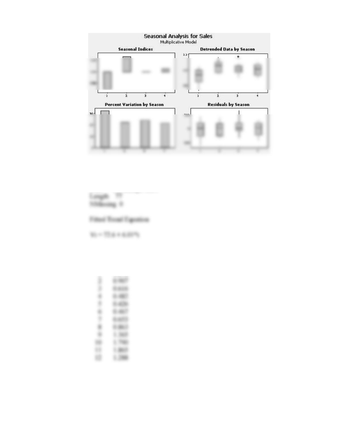
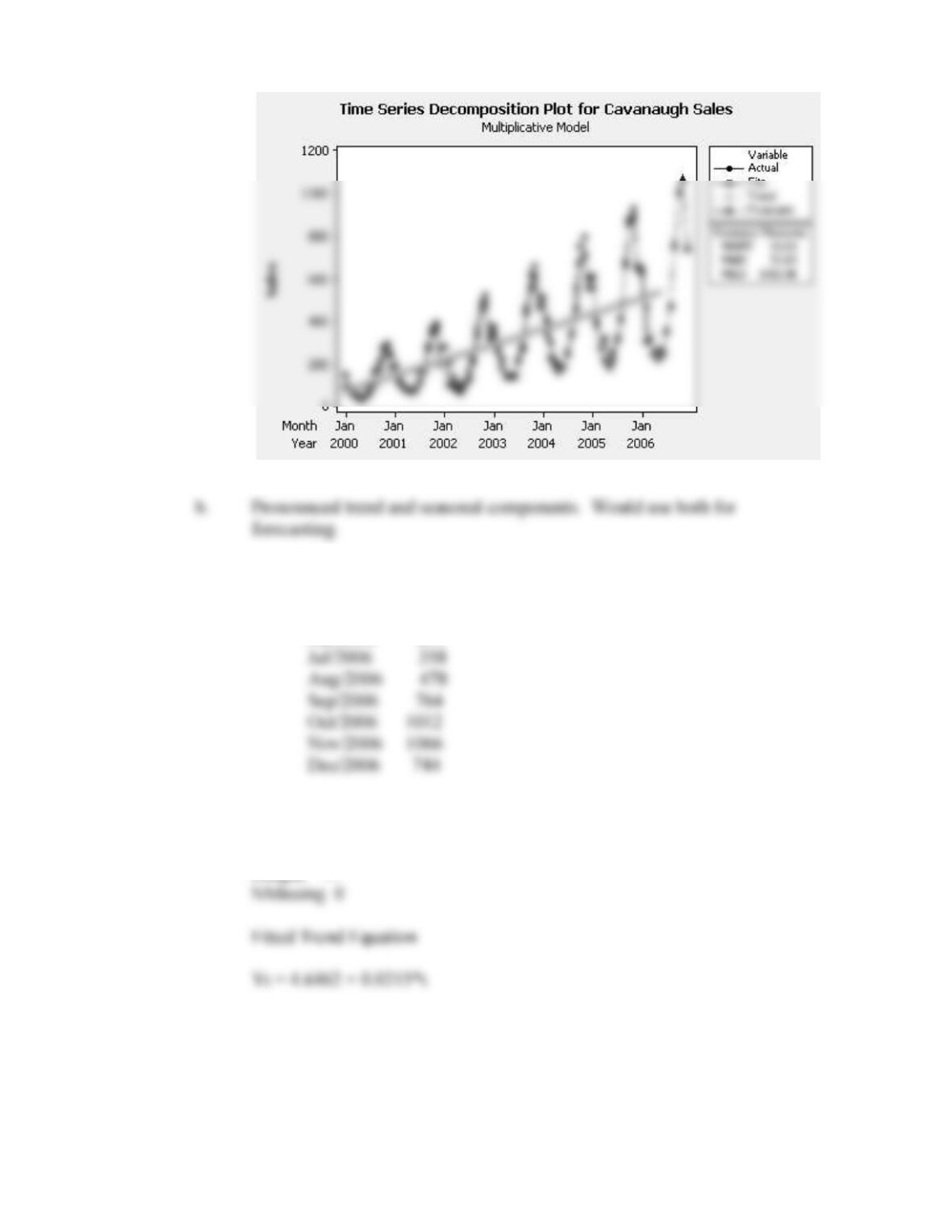
14. a. Multiplicative Model
Data Cavanaugh Sales
Seasonal Indices
Period Index
1 1.278
62
c. Forecasts (see plot in part a)
Month Forecast
Jun/2006 253
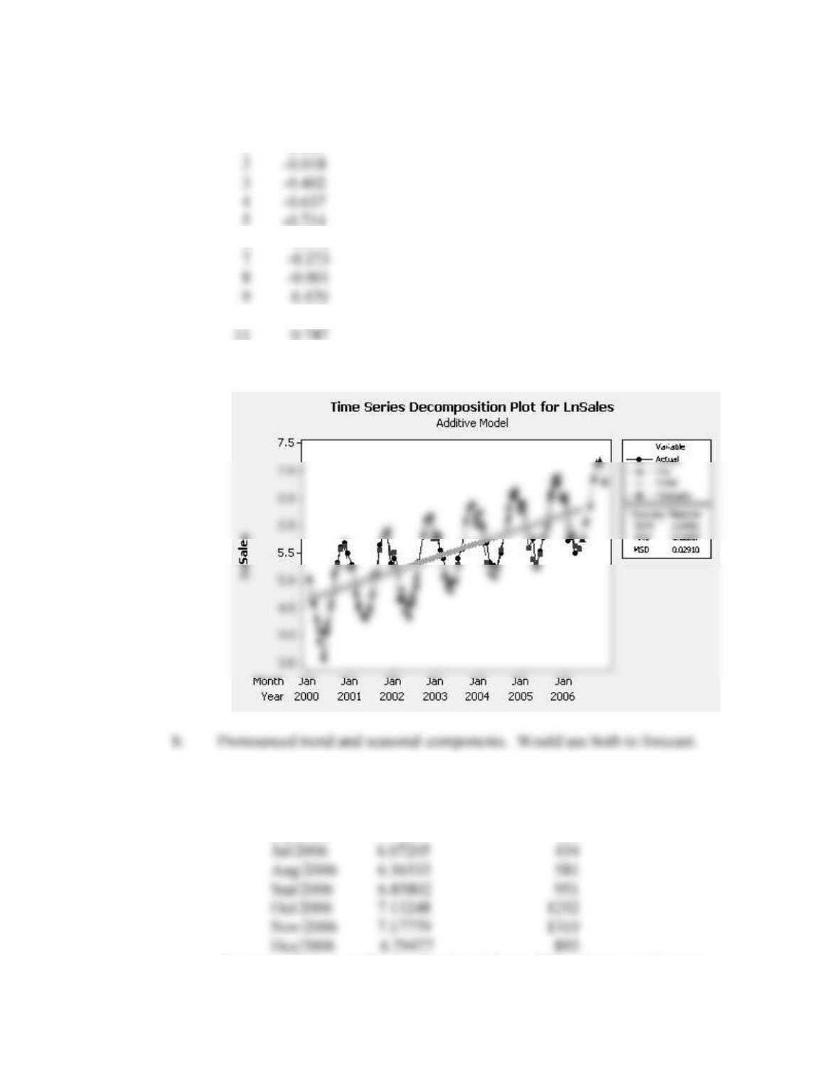
15. a. Additive Model
Data LnSales
Length 77
63
Seasonal Indices
Period Index
1 0.335
6 -0.571
10 0.723
12 0.342
c. & d. Forecasts
Month Forecast of LnSales Forecast of Sales
Jun/2006 5.75297 315
e. Forecasts of Cavanaugh sales developed from additive decomposition are
64
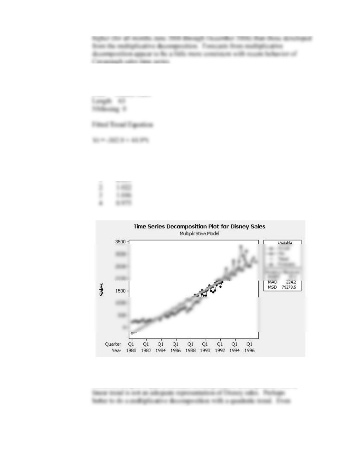
16. a. Multiplicative Model
Data Disney Sales
Seasonal Indices
Period Index
b. There is a significant trend but it is not a linear trend. First quarter sales
tend to be relatively low and third quarter sales tend to be relatively high.
However, the plot in part a indicates a multiplicative decomposition with a
65
d. Forecasts
Quarter Forecast
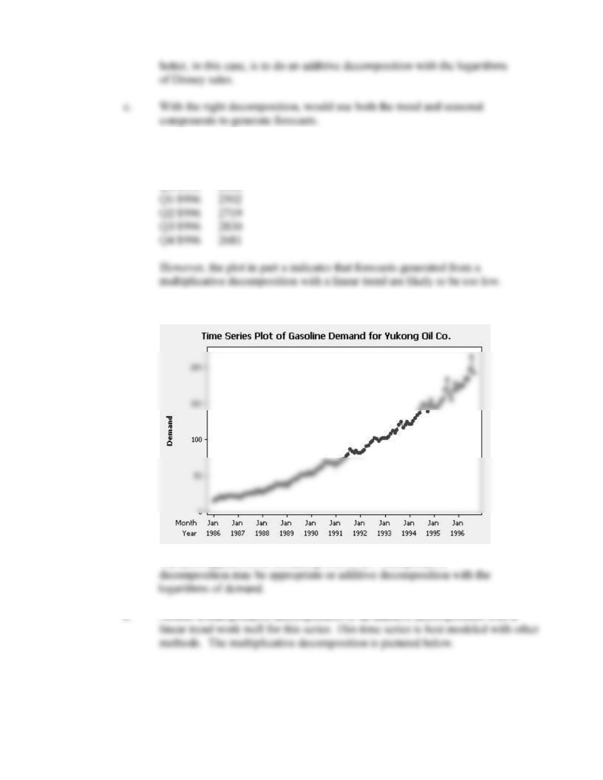
17. a.
Variation appears to be increasing with level. Multiplicative
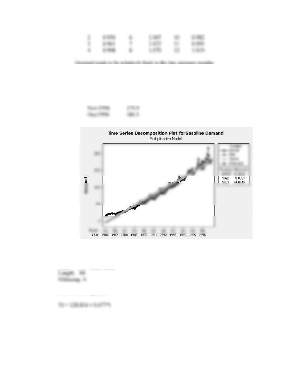
c. Seasonal Indices (Multiplicative Decomposition for Demand)
Period Index Period Index Period Index
66
1 0.947 5 1.004 9 1.045
Demand tends to be relatively high in the late summer months.
d. Forecasts derived from a multiplicative decomposition of demand (see plot
below).
Month Forecast
Oct/1996 171.2
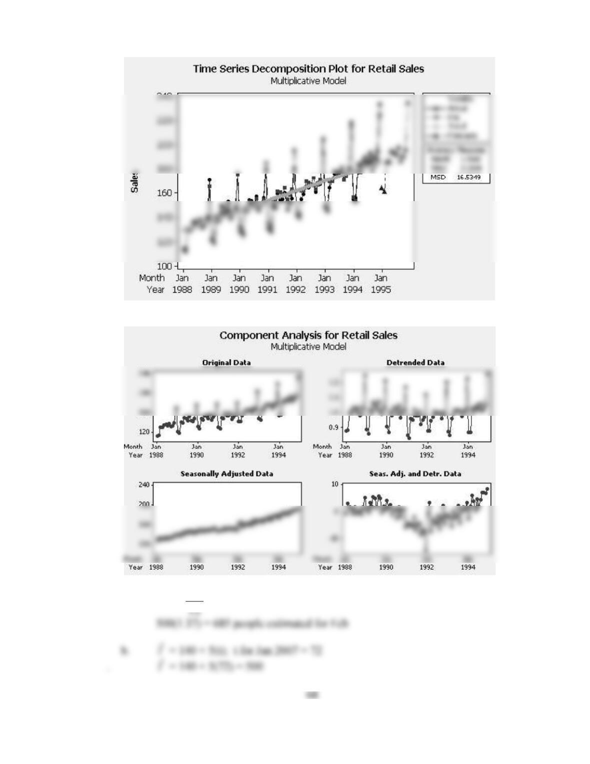
18. Multiplicative Model
Data U.S. Retail Sales
Fitted Trend Equation
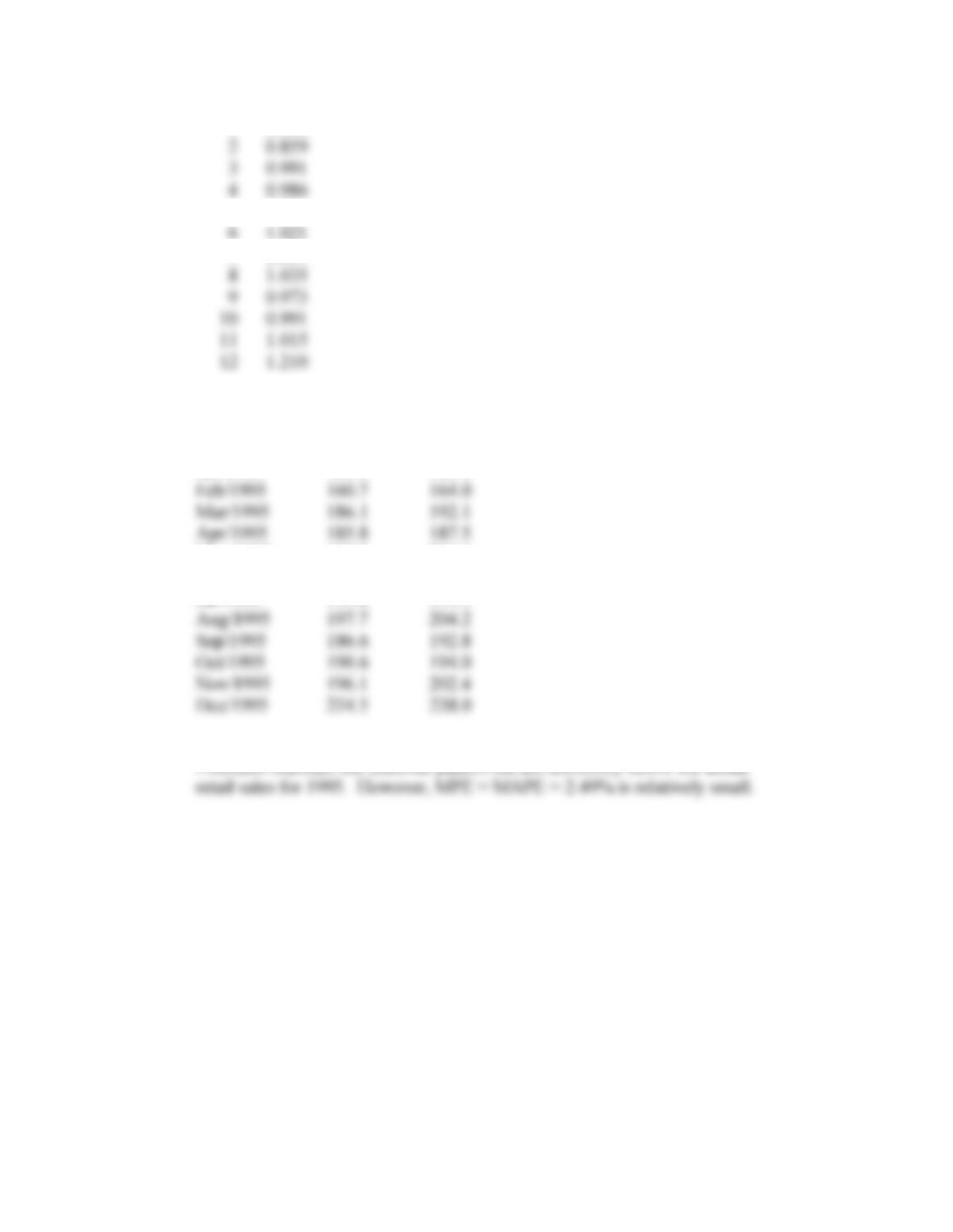
Seasonal Indices
67
Period Index
1 0.880
5 1.031
7 1.007
Forecasts and Actuals
Period Forecast Actual
Jan/1995 164.0 167.0
May/1995 194.9 201.4
Jun/1995 193.6 202.6
Jul/1995 191.8 194.9
19. a. Jan = 600
69
Jan
Y
= 500(1.20) = 600
22. Deflating a time series removes the effects of dollar inflation and permits the analyst
to examine the series in constant dollars.
24. Jan 303,589
Feb 251,254
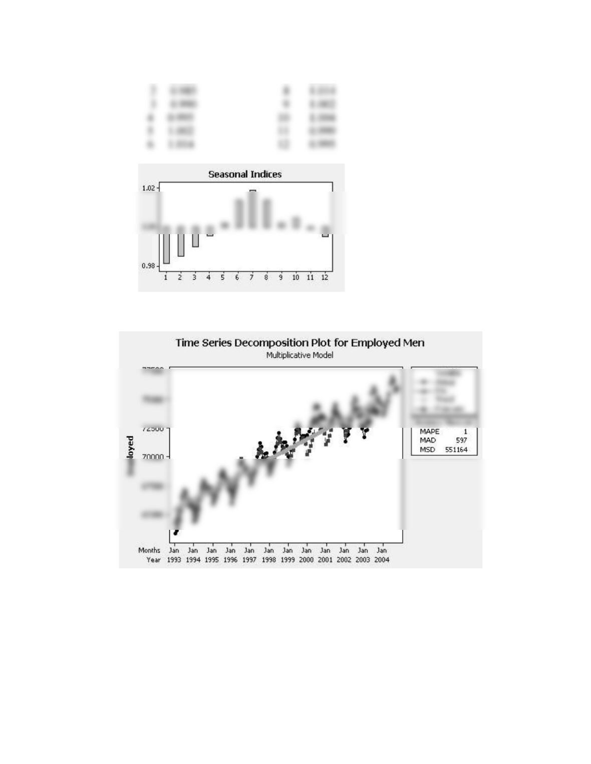
25. Multiplicative Model
Data Employed Men
Length 130
Seasonal Indices
Y
Y
Y
Y
Y
Y
Y
70
Month Index Month Index
1 0.981 7 1.019
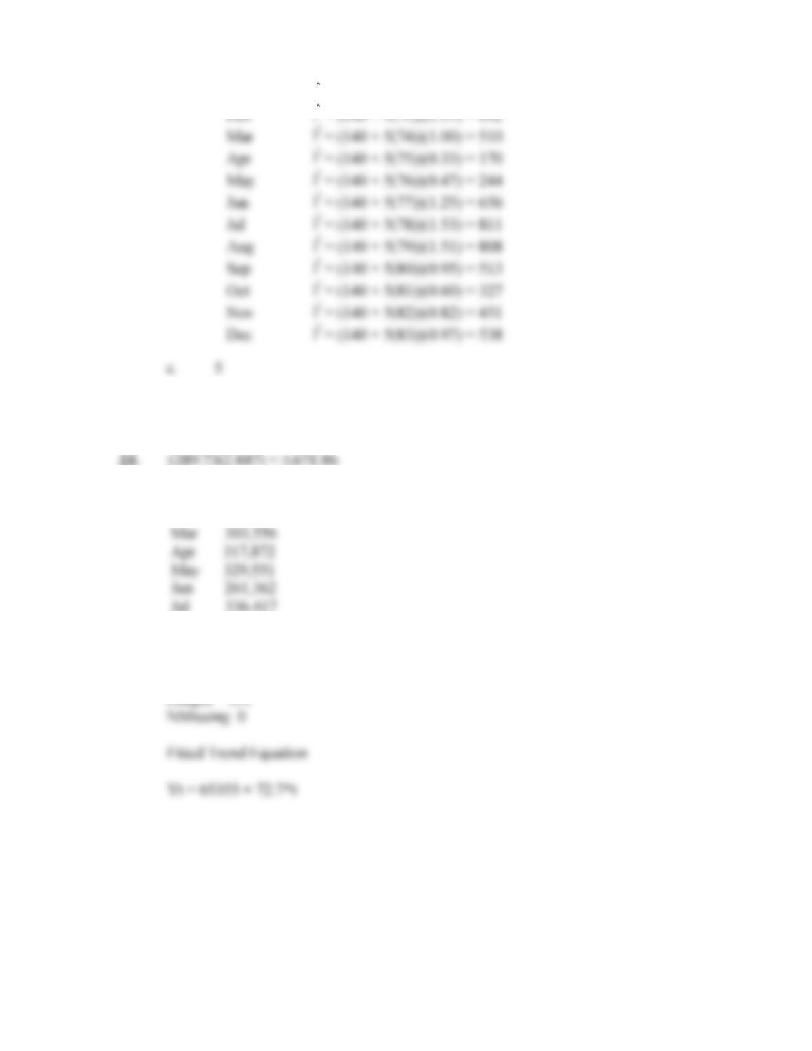
Forecasts
Month Forecast
Apr/2004 74887.2
May/2004 75454.0
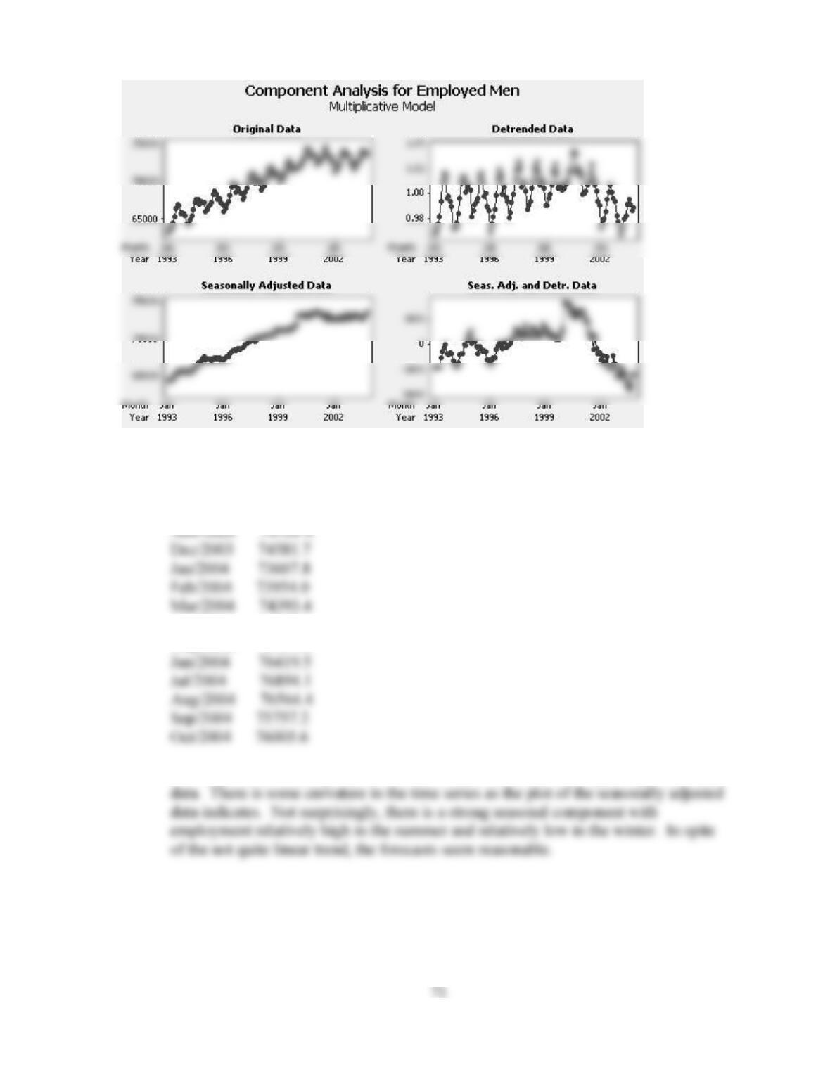
A multiplicative decomposition with a default linear trend is not quite right for these
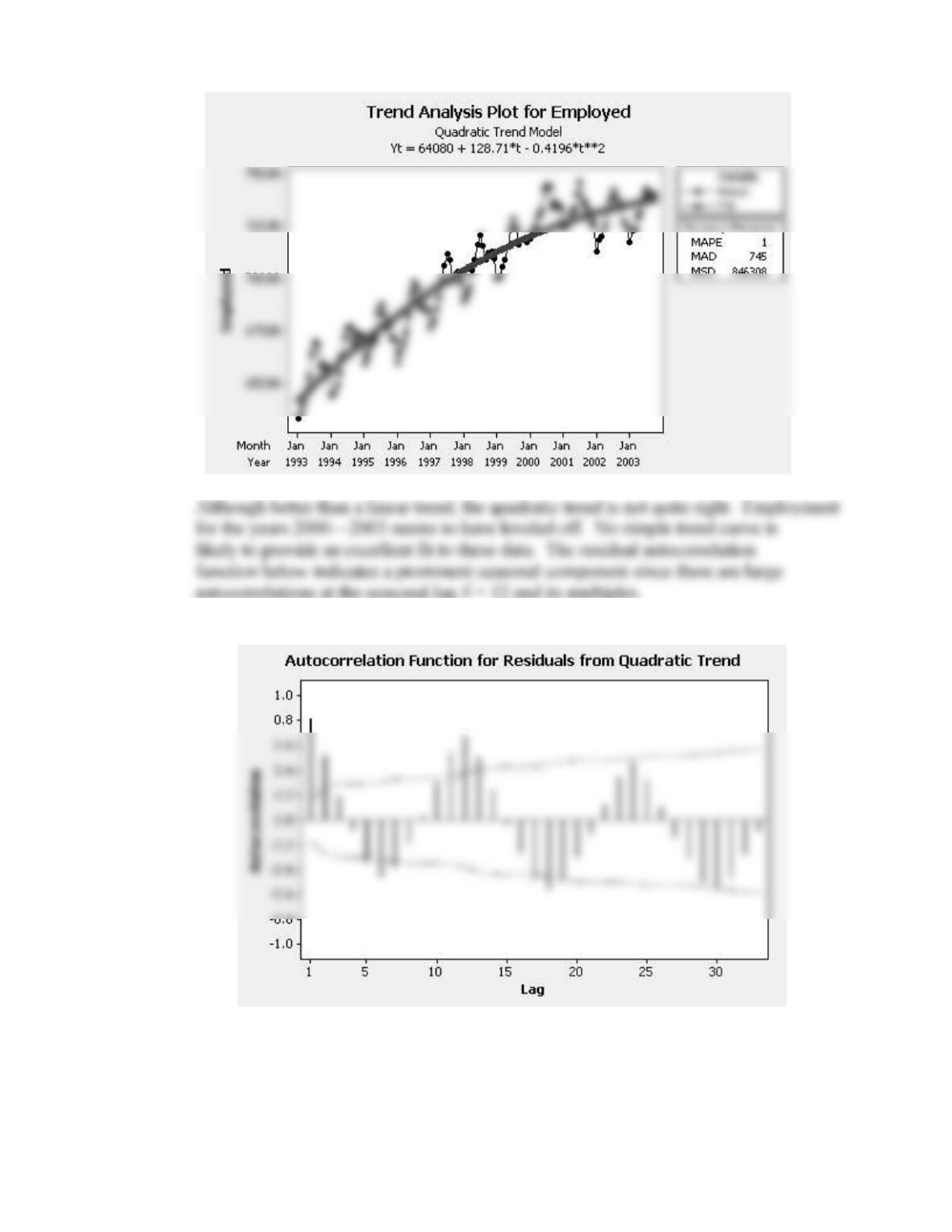
26. A linear trend is not appropriate for the employed men data. The plot below shows
a quadratic trend fit to the data of Table P-25.
72
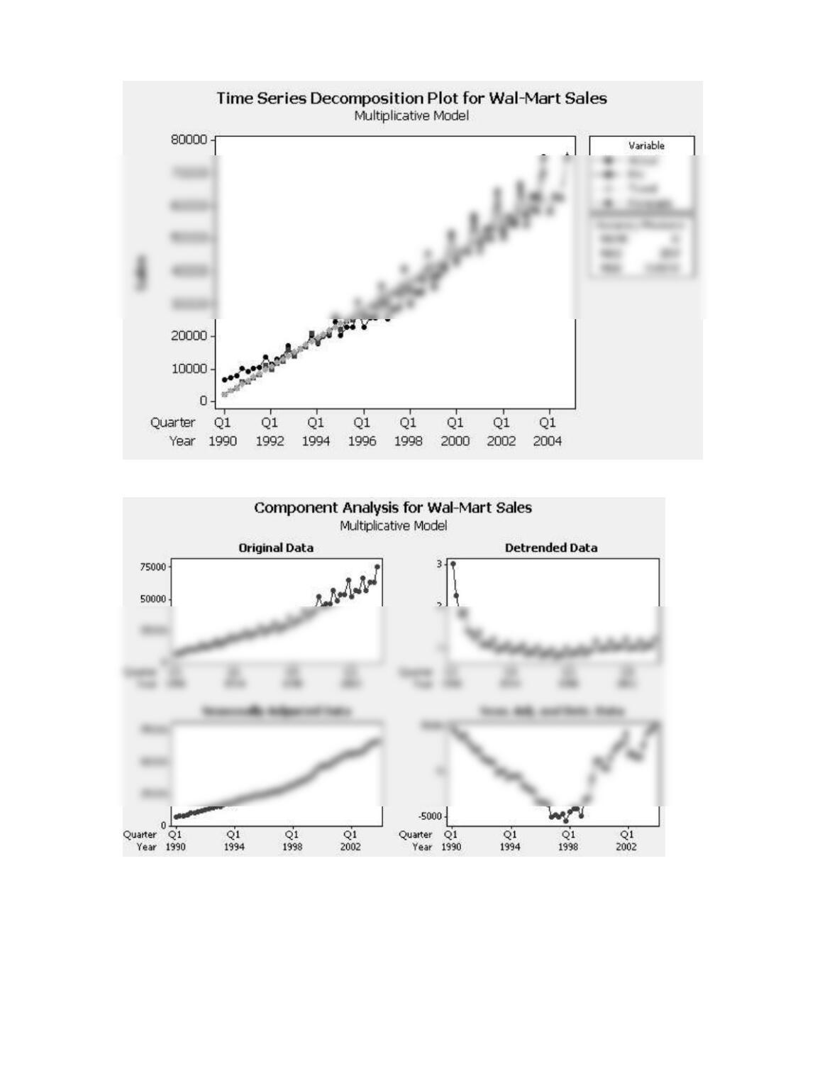
27. Multiplicative Model
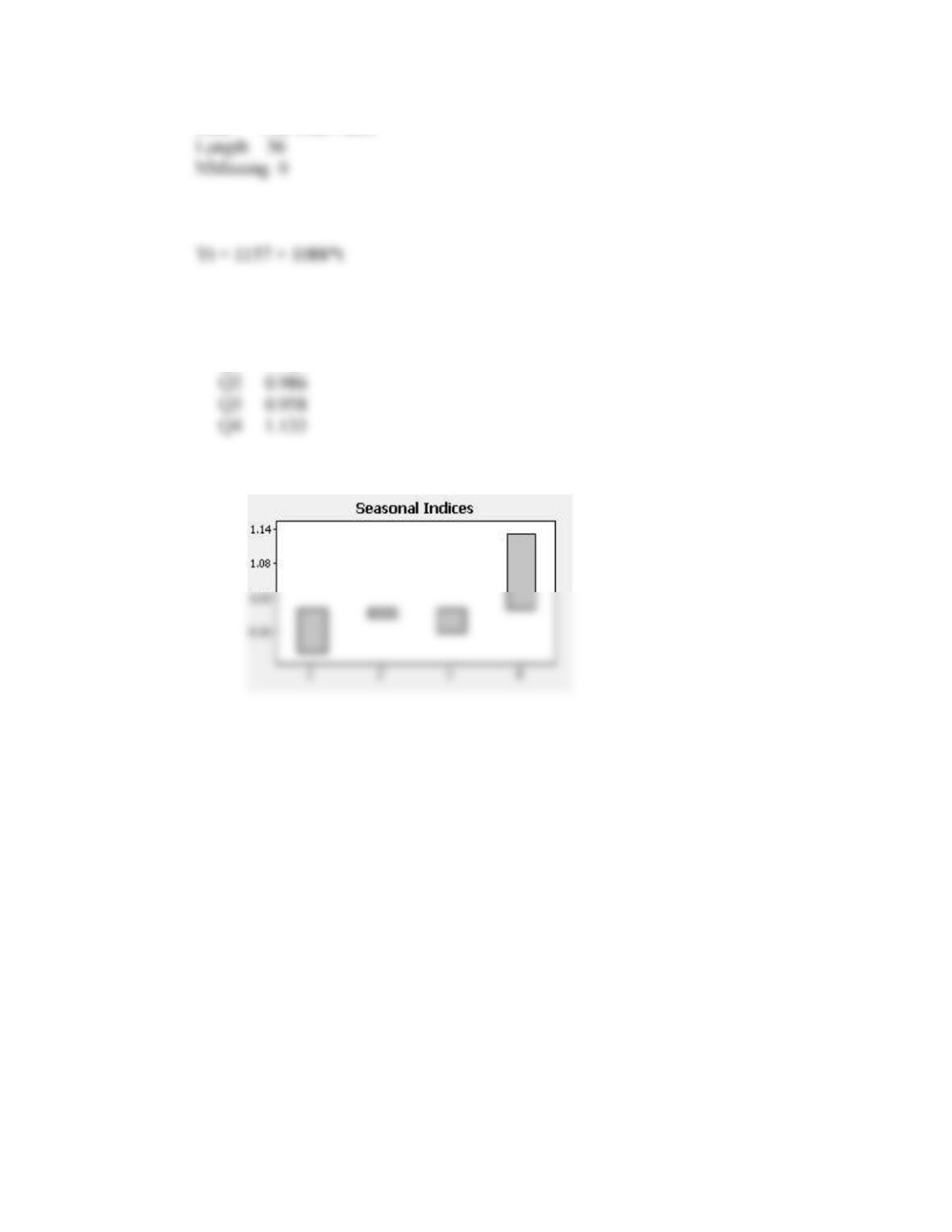
73
Data Wal-Mart Sales
Fitted Trend Equation
Seasonal Indices
Quarter Index
Q1 0.923
74
Forecasts and Actuals
Quarter Forecast Actuals
Q1/2004 58328 65443
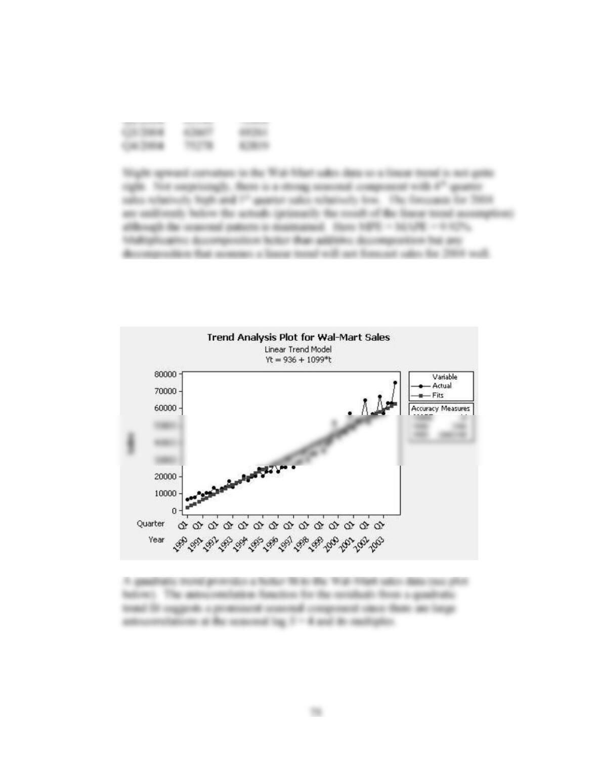
28. A linear trend fit to the Wal-Mart sales data of Table P-27 is shown below. A
linear trend misses the upward curvature in the data.