Neville’s Algorithm 1
5.2 Neville’s Algorithm
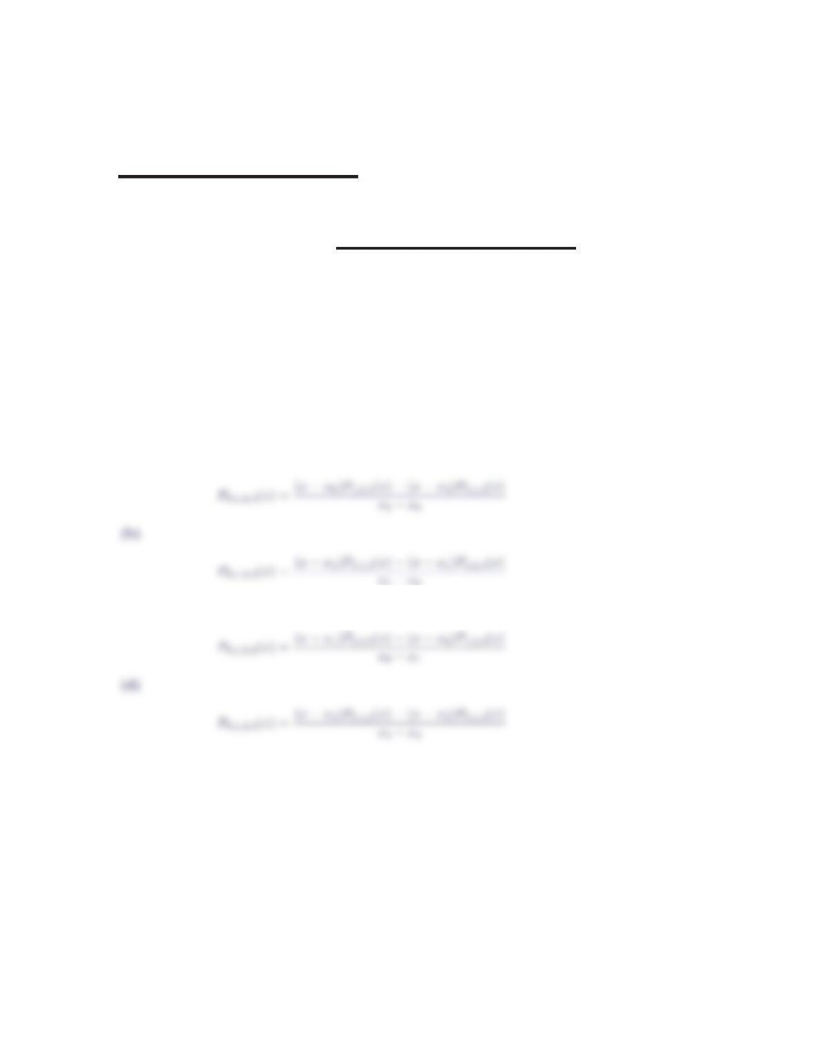
1. Indicate how to construct each of the following interpolating polynomials.
(a) P0,1,2,3(x) from P0,1,2(x) and P1,2,3(x)
(b) P0,1,2,3(x) from P0,2,3(x) and P0,1,3(x)
(c) P0,1,2,3(x) from P1,2,3(x) and P0,2,3(x)
(d) P0,1,2,3(x) from P0,1,3(x) and P0,1,2(x)
(a)
(c)
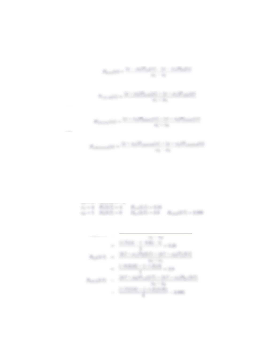
2. Indicate how to construct each of the following interpolating polynomials.
(a) P0,1,2(x) from P1,2(x) and P0,2(x)
(b) P1,3,4,6(x) from P1,4,6(x) and P1,3,6(x)
(c) P0,2,3,4,7(x) from P0,2,4,7(x) and P2,3,4,7(x)
(d) P1,2,3,4,5,6(x) from P1,2,3,5,6(x) and P1,3,4,5,6(x)
2Section 5.2
(a)
(b)
(c)
(d)
3. Construct the Neville’s table for the following data set. Take ¯x= 3.7.
x2 4 5
y−148
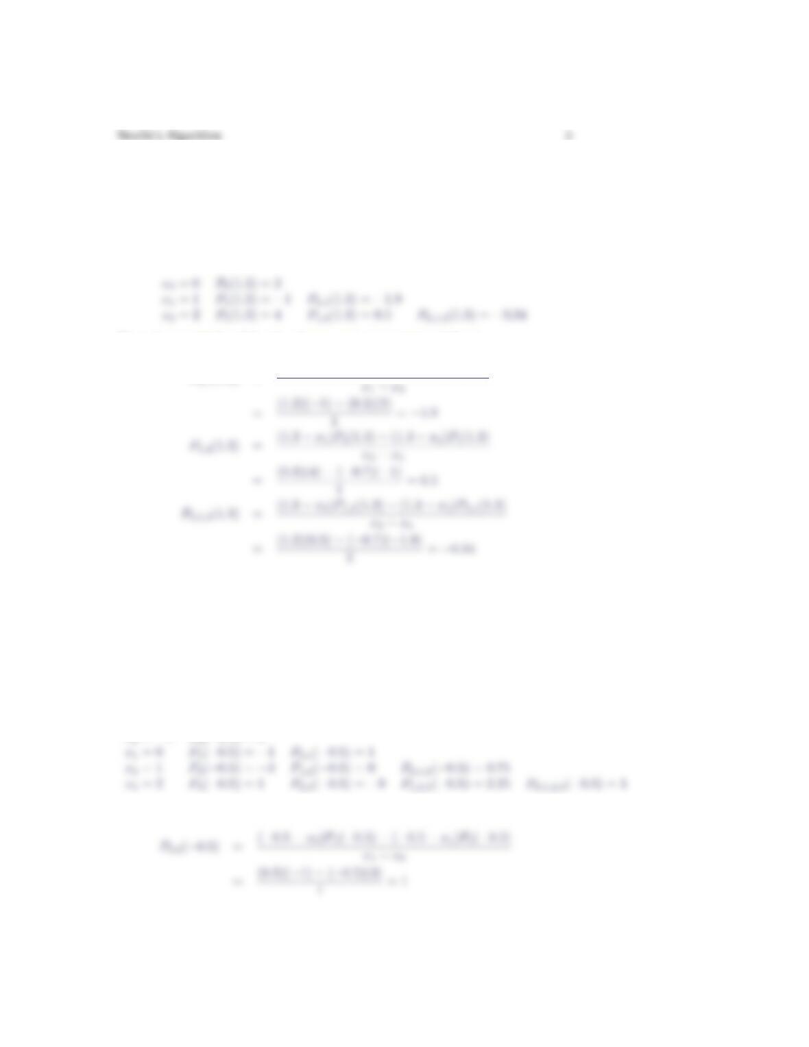
The complete Neville’s table is
The values in third and fourth columns were computed as follows:
P0,1(3.7) = (3.7−x0)P1(3.7) −(3.7−x1)P0(3.7)
4. Construct the Neville’s table for the following data set. Take ¯x= 1.3.
x0 1 2
y2−1 4
The complete Neville’s table is
The values in third and fourth columns were computed as follows:
P0,1(1.3) = (1.3−x0)P1(1.3) −(1.3−x1)P0(1.3)
5. Construct the Neville’s table for the following data set. Take ¯x=−0.5.
x−1 0 1 2
y3−1−3 1
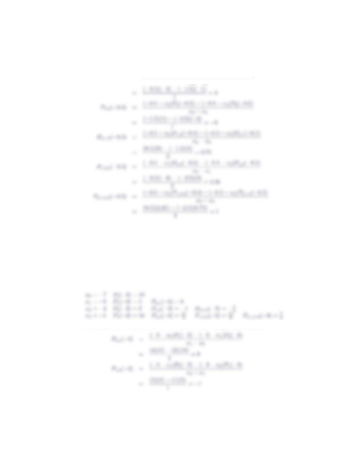
The complete Neville’s table is
x0=−1P0(−0.5) = 3
The values in the third, fourth and fifth columns were computed as follows:
4Section 5.2
P1,2(−0.5) = (−0.5−x1)P2(−0.5) −(−0.5−x2)P1(−0.5)
x2−x1
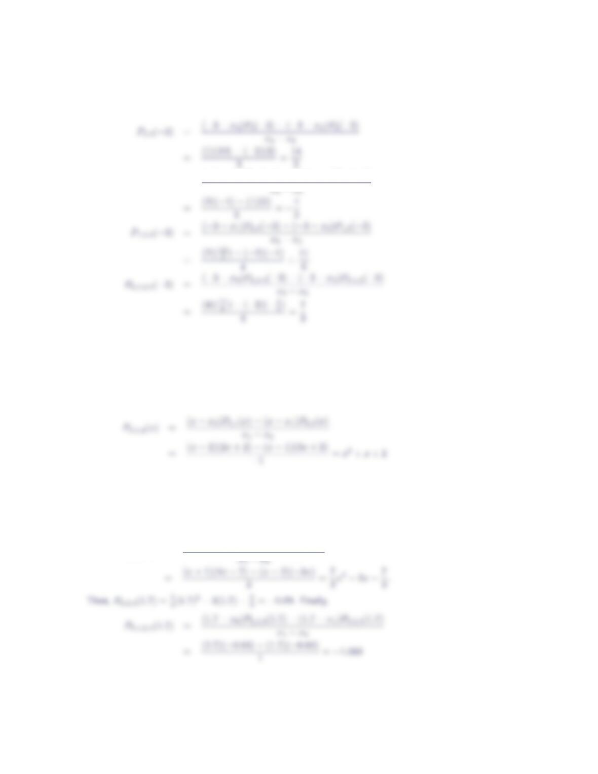
6. Construct the Neville’s table for the following data set. Take ¯x=−3.
x−7−5−4−1
y10 5 2 10
The complete Neville’s table is
The values in the third, fourth and fifth columns were computed as follows:
Neville’s Algorithm 5
P0,1,2(−3) = (−3−x0)P1,2(−3) −(−3−x2)P0,1(−3)
7. Given x0= 0, x1= 1, x2= 2, P0,1(x) = 2x+ 2 and P0,2(x) = 3x+ 2, what is
P0,1,2(x)?
To determine P0,1,2(x), we combine P0,1(x)and P0,2(x)as follows:
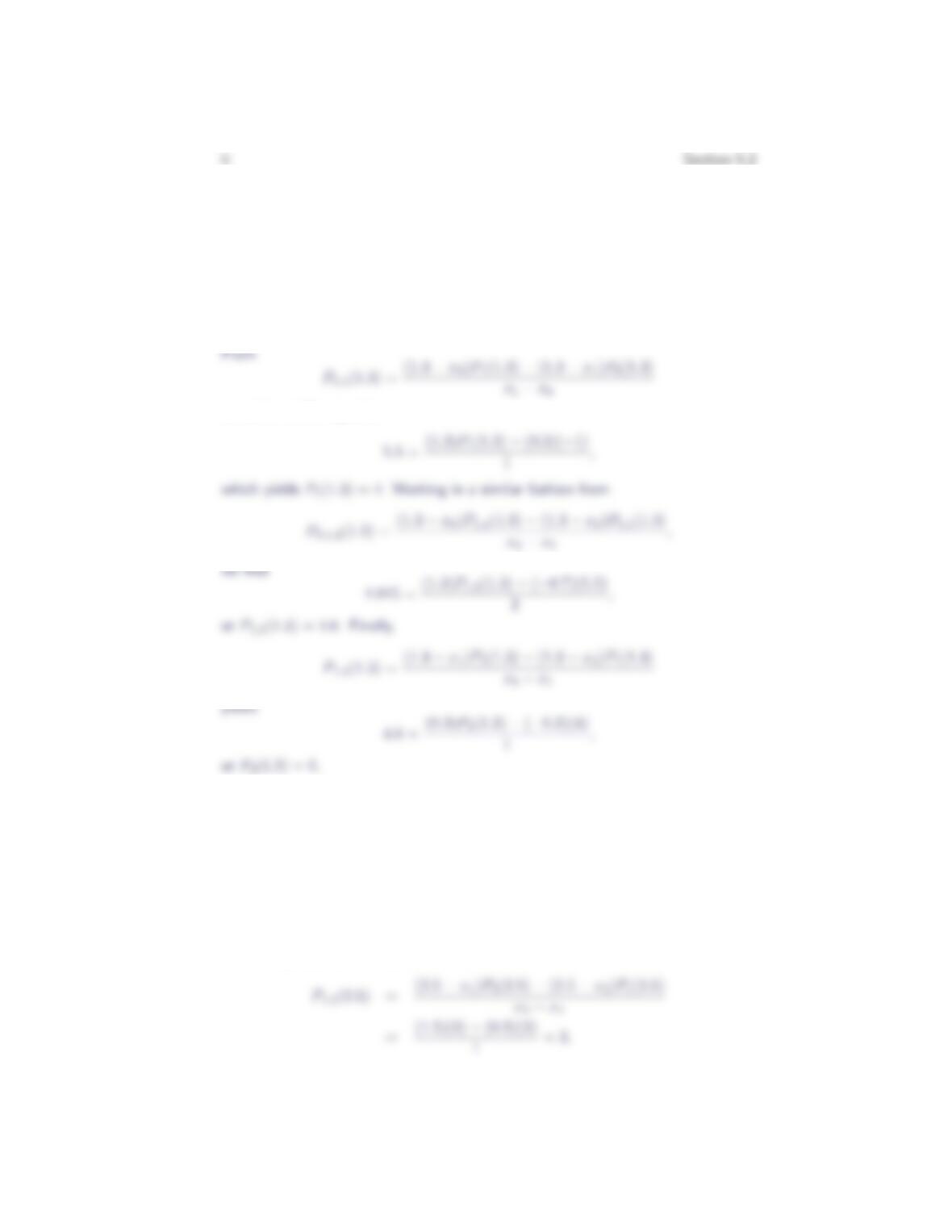
8. Given x0=−1, x1= 0, x2= 1, x3= 2, P0,2(x) = −3x,P2,3(x) = 4x−7 and
P1,2,3(1.7) = −0.83, calculate P0,2,3(x) and P0,1,2,3(1.7).
P0,2,3(x) = (x−x0)P2,3(x)−(x−x3)P0,2(x)
9. Determine the missing values in the Neville’s table provided below.
x0= 0 P0(1.3) = −1
x1= 1 P1(1.3) =? P0,1(1.3) = 5.5
x2= 2 P2(1.3) =? P1,2(1.3) =? P0,1,2(1.3) = 4.915
we arrive at the equation
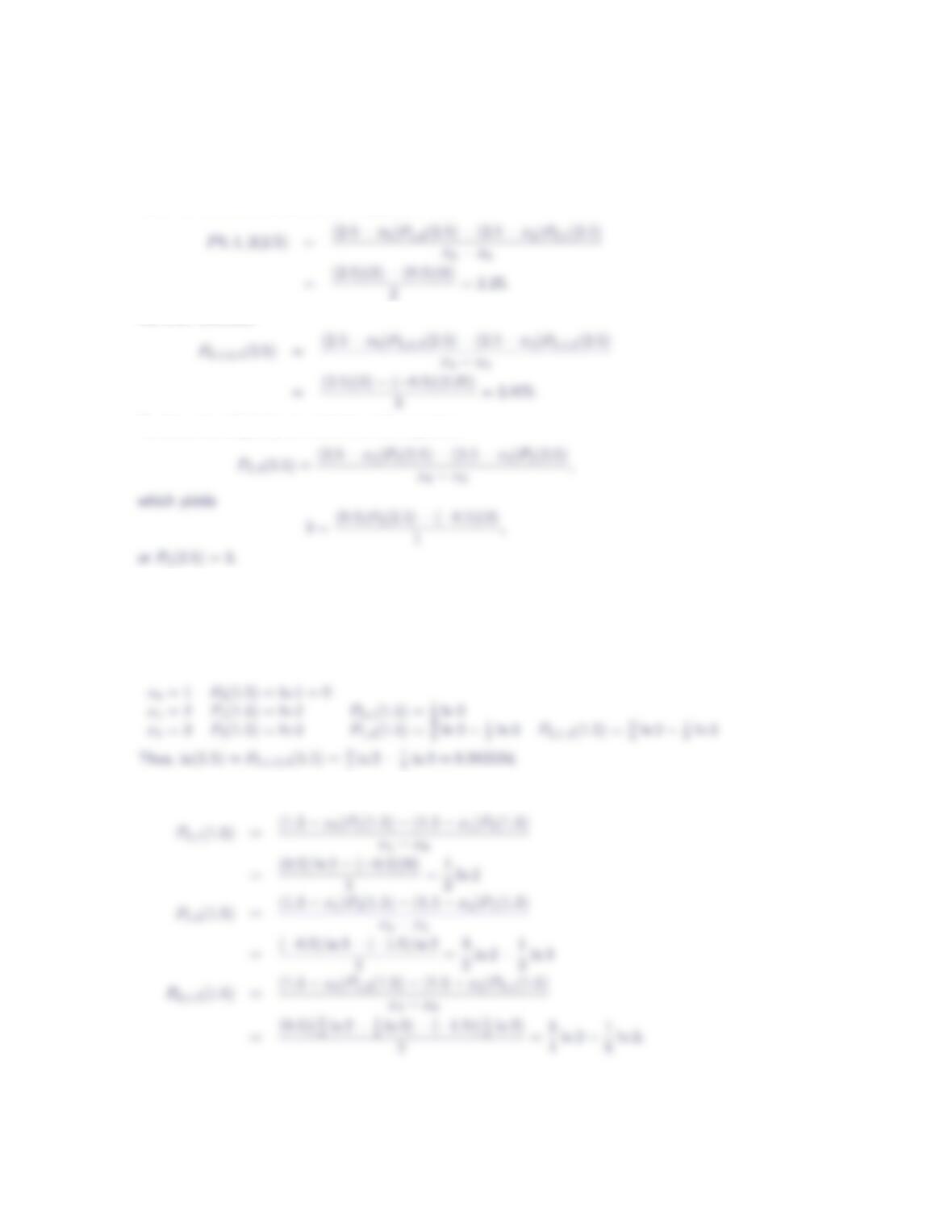
10. Determine the missing values in the Neville’s table provided below. For some
of the values you will need to work backwards.
x0= 0 P0(2.5) = 1
x1= 1 P1(2.5) = 3 P0,1(2.5) = 6
x2= 2 P2(2.5) = 3 P1,2(2.5) =? P0,1,2(2.5) =?
x3= 3 P3(2.5) =? P2,3(2.5) = 3 P1,2,3(2.5) = 3 P0,1,2,3(2.5) =?
Combining P1(2.5) and P2(2.5), we find
Neville’s Algorithm 7
Next, we combine P0,1(2.5) and P1,2(2.5) to find
We then calculate
To determine P3(2.5), we work from the equation
11. Use Neville’s algorithm to evaluate the interpolating polynomial for f(x) = ln x
which passes through the points (1,ln 1), (2,ln 2) and (3,ln 3) at x= 1.5.
The complete Neville’s table is
The values in the third and fourth columns were computed as follows:
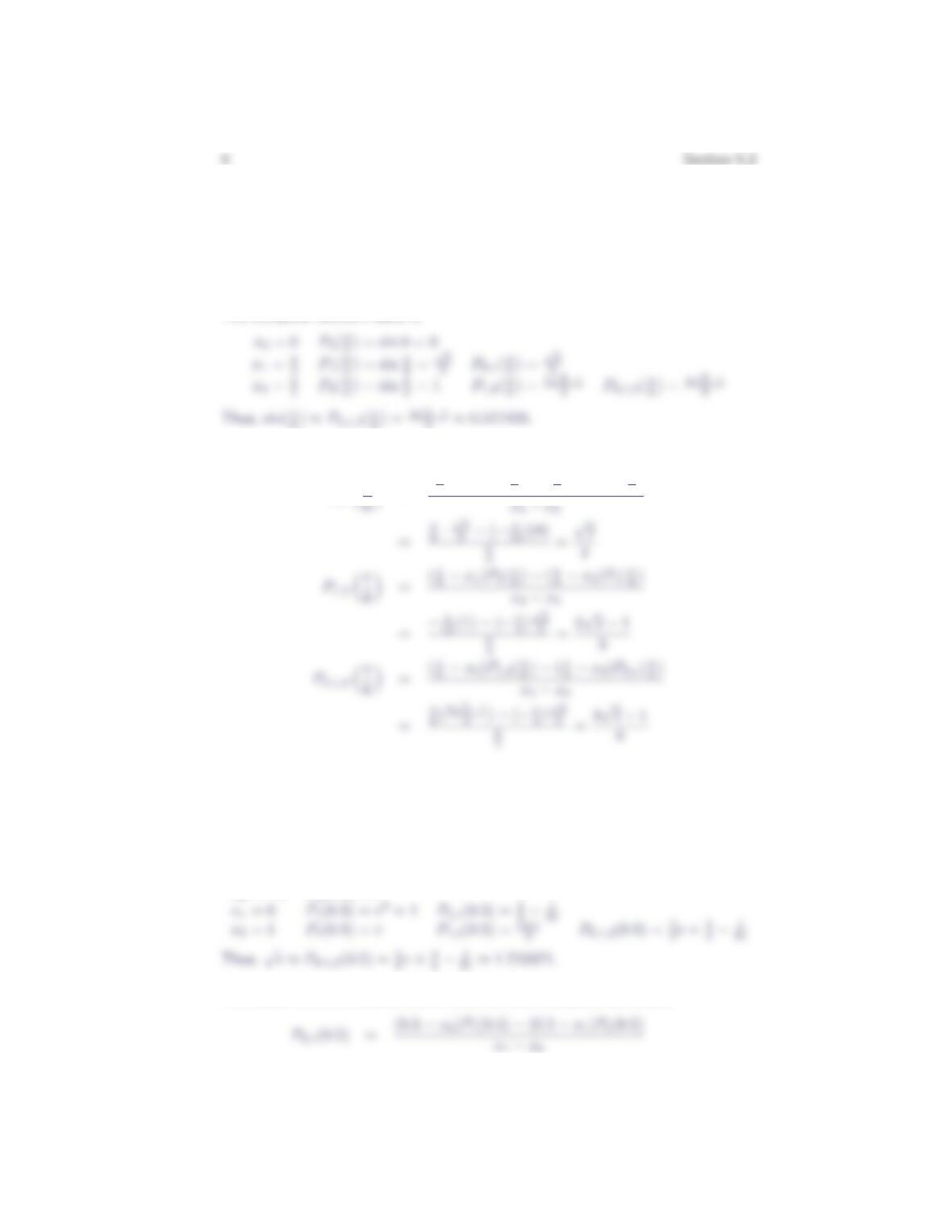
12. Use Neville’s algorithm to evaluate the interpolating polynomial for f(x) = sin x
which passes through the points (0,sin 0), (π/4,sin π/4) and (π/2,sin π/2) at
x=π/6.
The complete Neville’s table is
The values in the third and fourth columns were computed as follows:
P0,1π
6−x0)P1(π
6)−(π
6−x1)P0(π
6)
13. Use Neville’s algorithm to evaluate the interpolating polynomial for f(x) = ex
which passes through the points (−1, e−1), (0, e0) and (1, e1) at x= 0.5.
The complete Neville’s table is
x0=−1P0(0.5) = e−1
The values in the third and fourth columns were computed as follows:
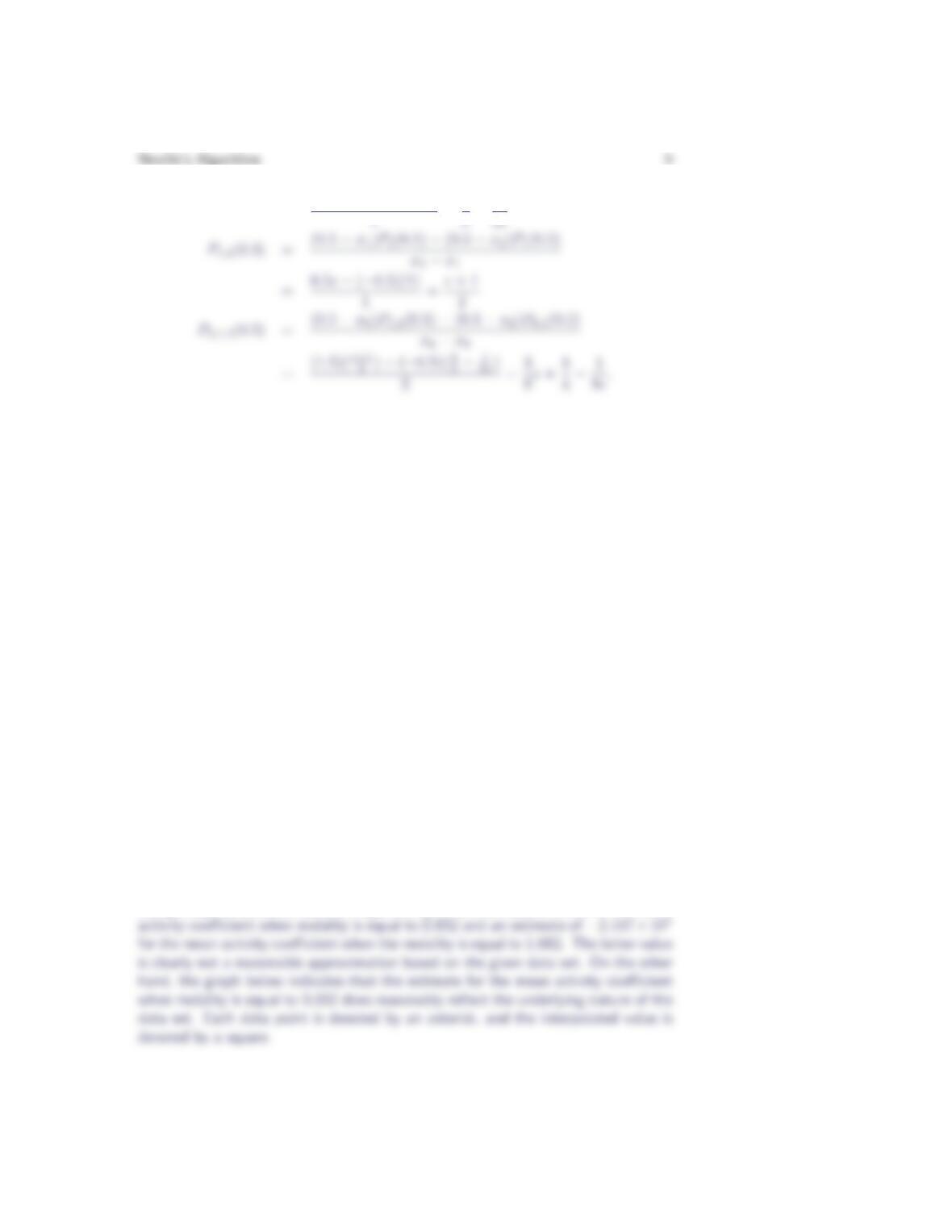
=(1.5)(1) −(0.5)e−1
For Exercises 14 – 17, use Neville’s algorithm to estimate the requested value(s).
Assess the accuracy of each estimate by plotting the data points and the esti-
mated point(s) on the same set of coordinate axes.
14. The mean activity coefficient at 25◦C for silver nitrate, as a function of molality,
is given in the table below. Estimate the mean activity coefficient for a molality
of 0.032 and for a molality of 1.682.
molality 0.005 0.010 0.020 0.050 0.100 0.200 0.500 1.000 2.000
coefficient 0.924 0.896 0.859 0.794 0.732 0.656 0.536 0.430 0.316
Using the given data set, Neville’s algorithm gives an estimate of 0.831 for the mean
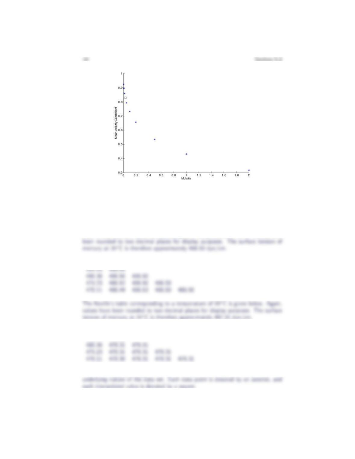
15. The values listed in the table provide the surface tension of mercury as a function
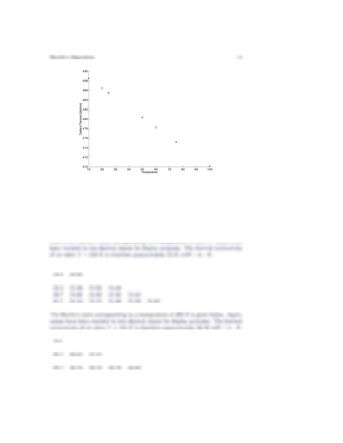
of temperature. Estimate the surface tension of mercury at 20◦C and at 60◦C.
Temperature (◦C) 10 25 50 75 100
Surface Tension (dyn/cm) 488.55 485.48 480.36 475.23 470.11
Here is the Neville’s table corresponding to a temperature of 20◦C. Values have
488.55
488.55
485.48 478.32
The following graph suggests that both interpolated values reasonably reflect the
16. The thermal conductivity of air as a function of temperature is given in the
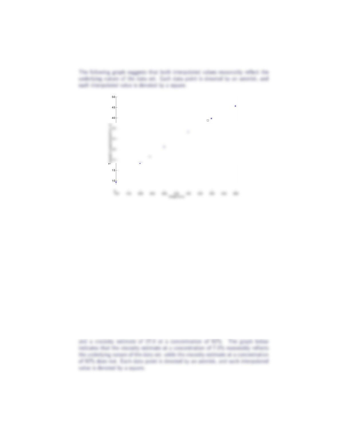
table below. Estimate the thermal conductivity of air when T=240K and when
T=485K.
Temperature (K) 100 200 300 400 500 600
Thermal Conductivity (mW/m·K) 9.4 18.4 26.2 33.3 39.7 45.7
9.4
26.2 21.52 21.66
45.7 24.10 22.23 21.48 21.59 21.62
18.4 44.05
33.3 39.34 38.78 39.16
45.7 38.80 38.77 38.77 38.78 38.78
12 Section 5.2
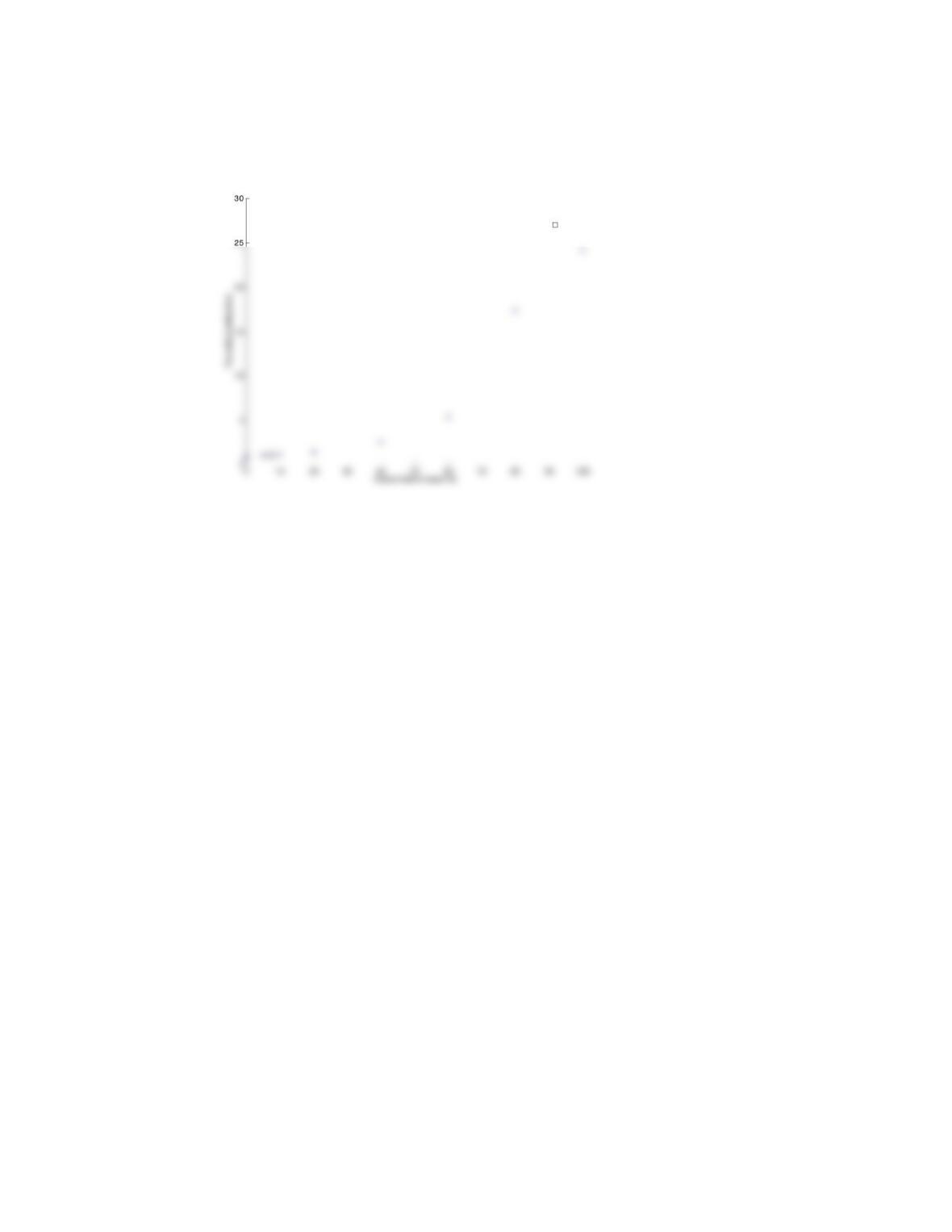
17. Estimate the viscosity of sulfuric acid with a concentration (in mass percent) of
7.5% and a concentration of 92% given the following values.
Concentration (mass %) 0 5 10 20 40 60 80 100
Viscosity (centipoise) 0.89 1.01 1.12 1.40 2.51 5.37 17.4 24.2
Neville’s algorithm produces a viscosity estimate of 1.07 at a concentration of 7.5%
Neville’s Algorithm 13