77
CASE 5-1: THE SMALL ENGINE DOCTOR
1.
2.
78
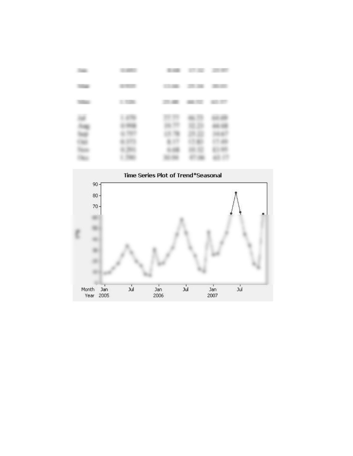
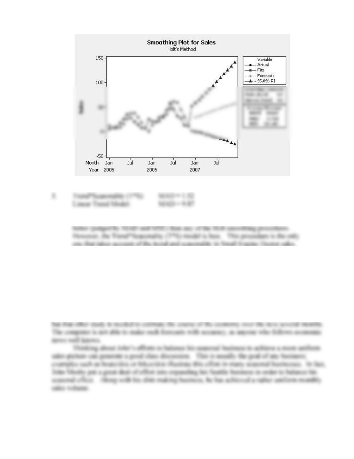
3. SEASONAL FITTED VALUES AND
ADJUSTMENT FORECASTS, T*S
MONTH FACTORS 2005 2006 2007
Feb 0.707 9.59 18.41 27.23
Apr 1.142 17.87 32.13 46.38
Jun 1.940 34.39 58.61 82.82
79
4.
80
6. If you had to limit your choices to the models in 2 and 4, the linear trend model is
CASE 5-2: MR. TUX
At last, John is able to deal directly with the strong seasonal effect in his monthly data.
Students find it interesting that in addition to using these to forecast, John’s banker wants them to
justify variable loan payments.
To forecast using decomposition, students see that both the C and I components must be
estimated. We like to emphasize that studying the C column in the computer printout is helpful,

81
1. The two sentences might look something like this: A computer analysis of John
2. Since John expects to do twice as much business in Seattle as Spokane, the Seattle
indices he should try to achieve will be only half as far from 100 as the Spokane
indices, and on the opposite side of 100:
Spokane Seattle
Feb 47.2 126.4
Apr 177.9 61.1
Jun 118.6 90.7
Aug 128.7 85.7
3.
dollars, divide the actual sales by the corresponding seasonal index:
Now subtract the actual sales from these target values to get the sales necessary
from the shirt making machine:
CASE 5-3: CONSUMER CREDIT COUNSELING
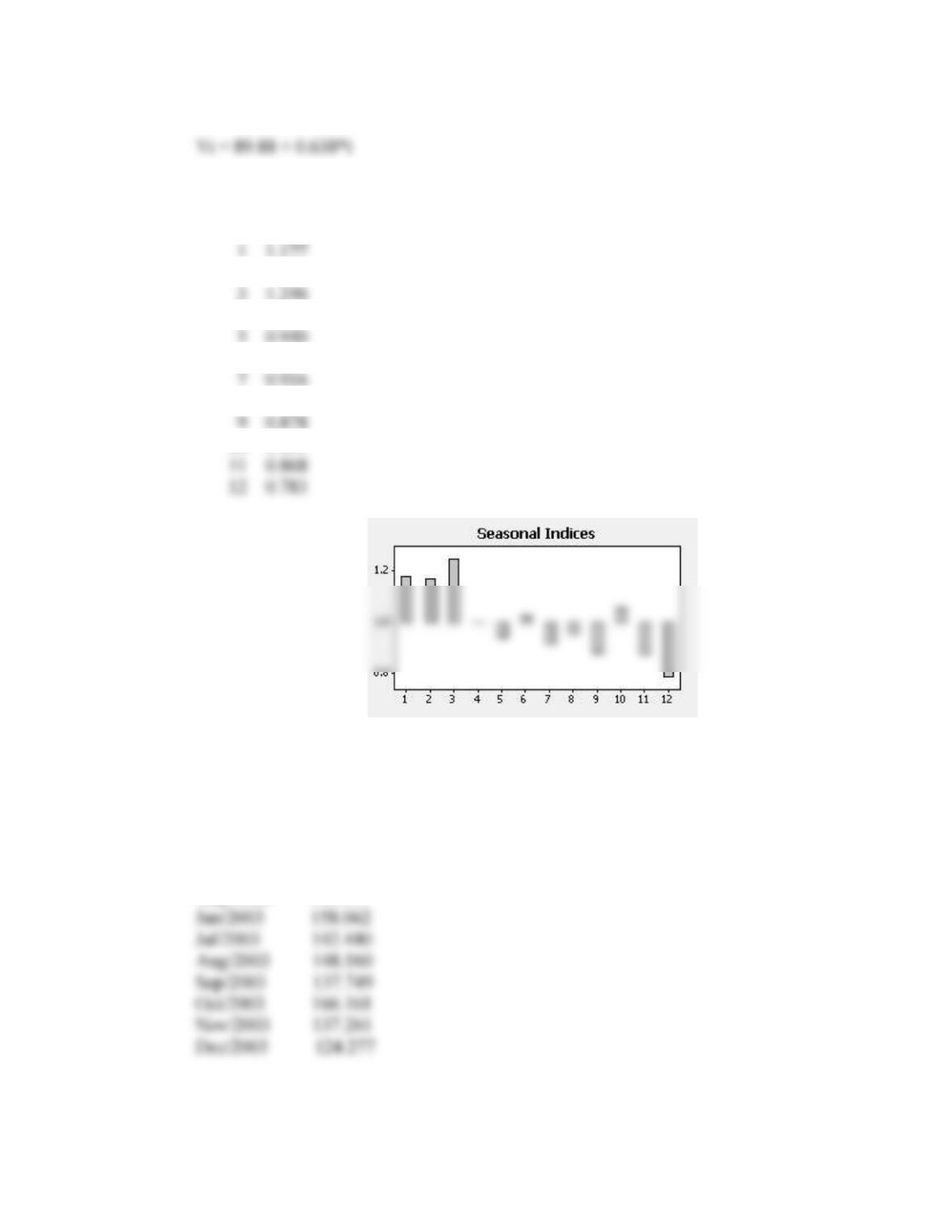
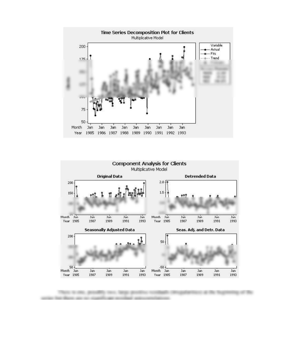
Both the trend and seasonal components are important. The trend explains about 34%
percent of the total variance.
Multiplicative Model
Data Clients
Length 99
82
Fitted Trend Equation
Seasonal Indices
Month Index
2 1.168
4 0.997
6 1.020
8 0.951
10 1.055
The number of new clients tends to be relatively large during the first three months
of the year.
Forecasts
Month Forecast
Apr/2003 153.207
May/2003 145.121
83
CASE 5-4: MURPHY BROTHERS FURNITURE
84
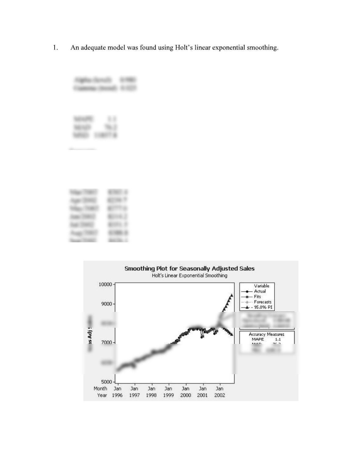
Smoothing Constants
Accuracy Measures
Forecasts
Month Forecast
Jan/2002 8127.8
Feb/2002 8165.1
Sep/2002 8426.1
2. Forecasts and Actuals
85
Month Forecast Actual
Jan/2002 7453.2 7120
Feb/2002 7462.5 7124
2002.
CASE 5-5: AAA WASHINGTON
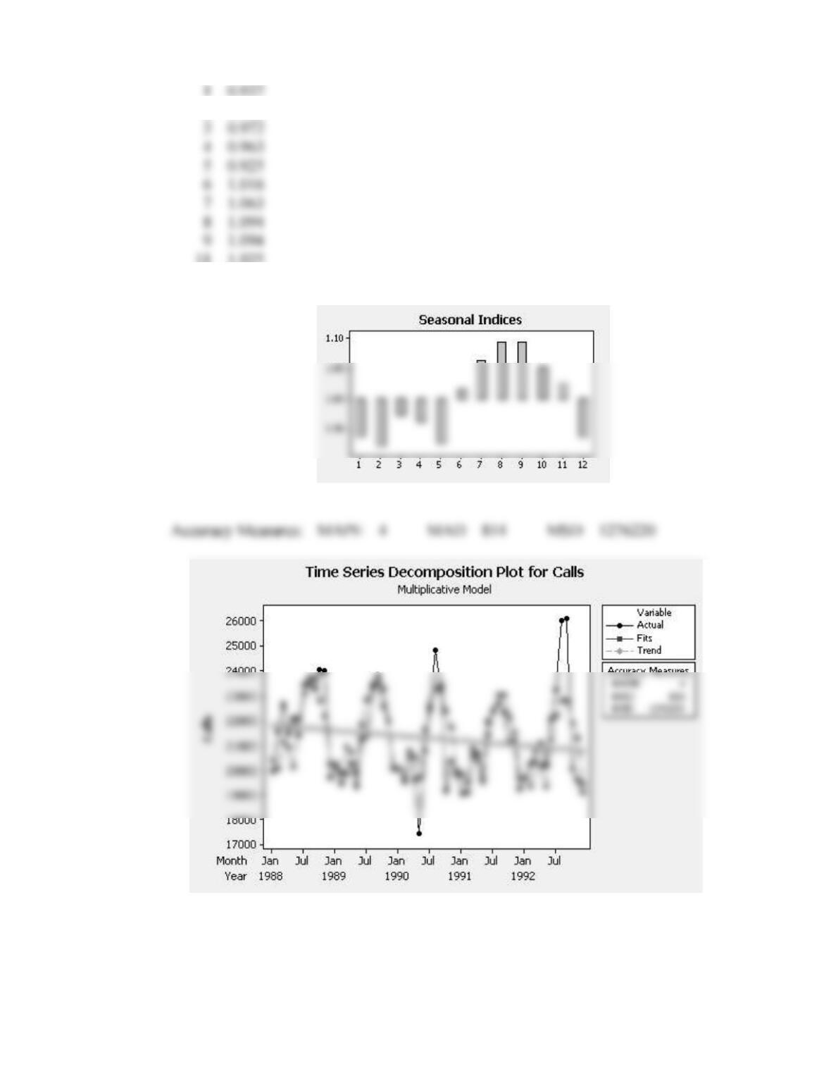
1. An additive and a multiplicative decomposition perform equally well. The multiplicative
decomposition is shown below.
Multiplicative Model
Data Calls
Seasonal Indices
Month Index
86
2 0.922
11 1.025
12 0.936
87
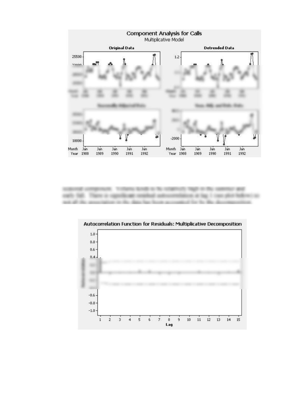
2. Decomposition analysis works pretty well for AAA Washington data. There is a
slight downward trend in emergency road service call volume with a pronounced
CASE 5-6: ALOMEGA FOOD STORES
88
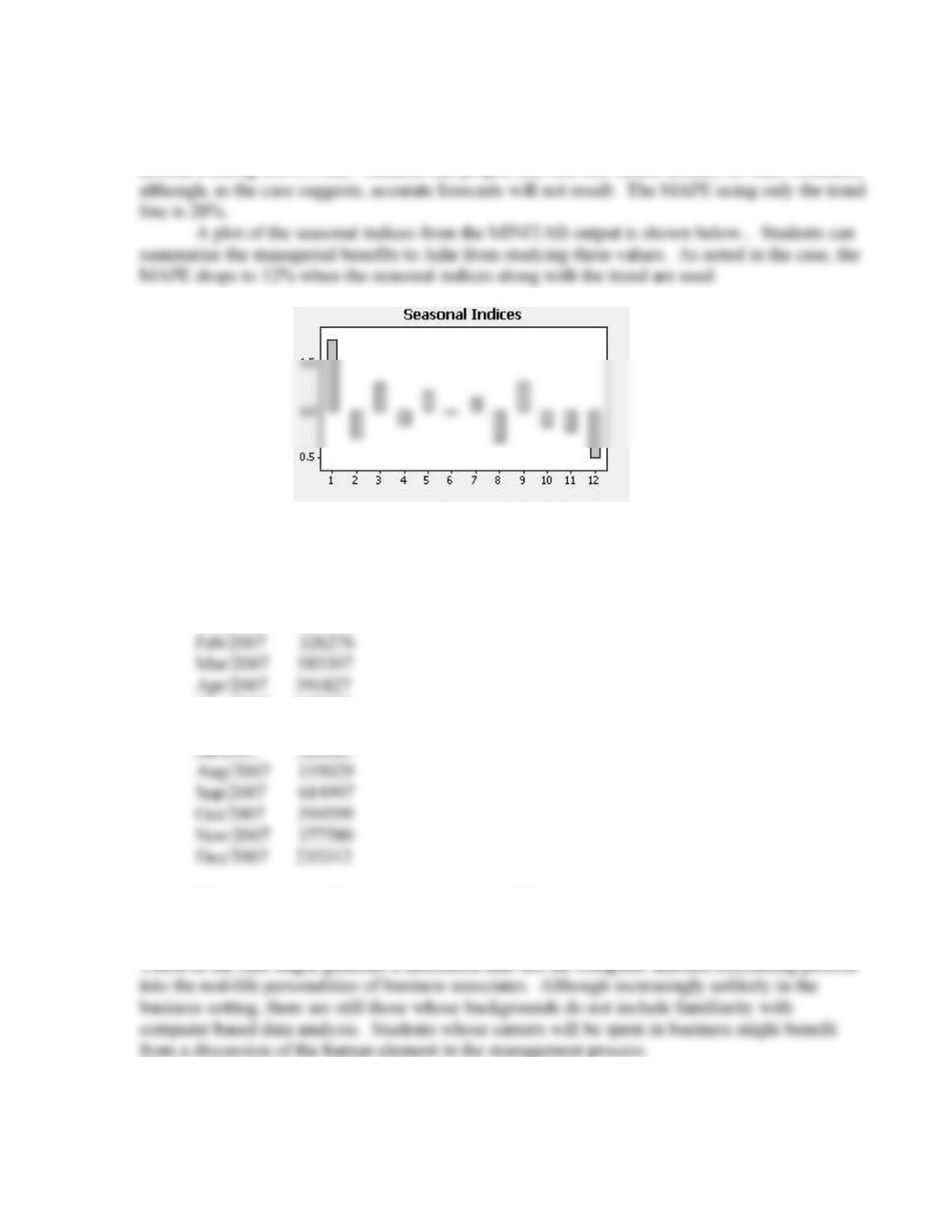
The sales data for the Alomega Food Stores case is subjected to a multiplicative
decomposition procedure in this case. A trend line is first calculated with the actual data plotted
around it (using MINITAB). Students can project this line into future months for sales forecasts,
Finally, a 12-month forecast is generated using both the trend line and the seasonal
indices. The forecasts seem reasonable.
Month Forecast
Jan/2007 785348
May/2007 558299
Jun/2007 453257
There are no significant residual autocorrelations.
Although more a management concern than a forecasting one, the attitude of Jackson
CASE 5-7: SURTIDO COOKIES
89
1. Multiplicative Model
Data SurtidoSales
Seasonal Indices
Month Index
1 0.696
7 0.716
90
Month Forecast
Jun/2003 680763
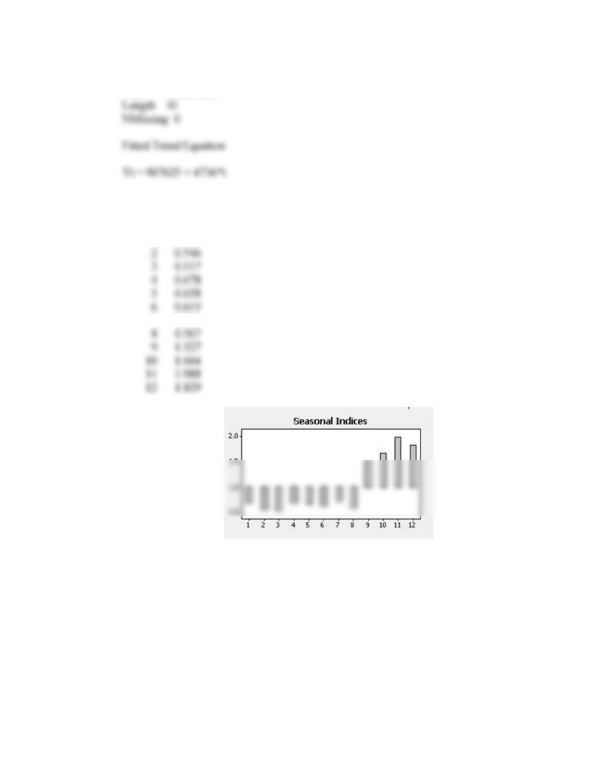
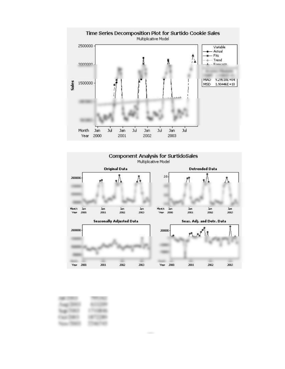
2. The linear trend in sales has a slight upward slope. The seasonal indices show that
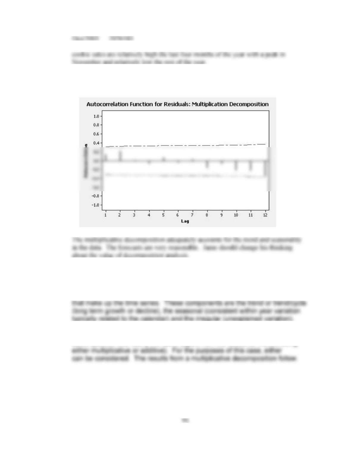
3. The residual autocorrelation function is shown below. There are no significant
residual autocorrelations.
CASE 5-8: SOUTHWEST MEDICAL CENTER
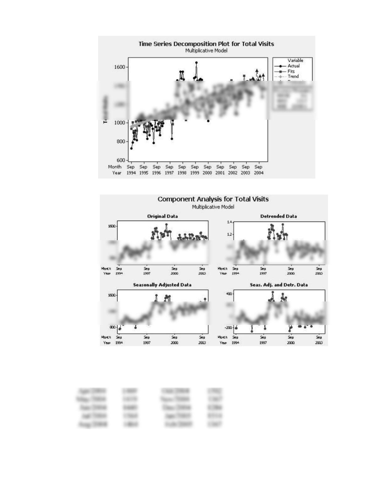
1. Decomposition of a time series involves isolating the underlying components
2. The results and forecasts from a multiplicative decomposition and an additive
decomposition are nearly the same (apart from the seasonal indices being
92
Multiplicative Model
Data Total Visits
Seasonal Indices
Month Index
1 0.972
3 0.943
5 1.039
7 1.043
93
Forecasts
Month Forecast Month Forecast
Mar/2004 1479 Sep/2004 1401
94
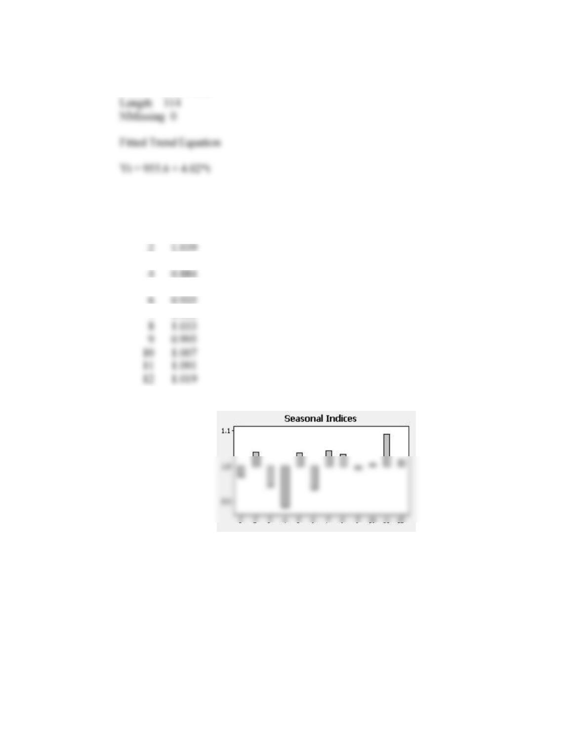
3. There is a distinct upward trend in total visits. The seasonal indices show that
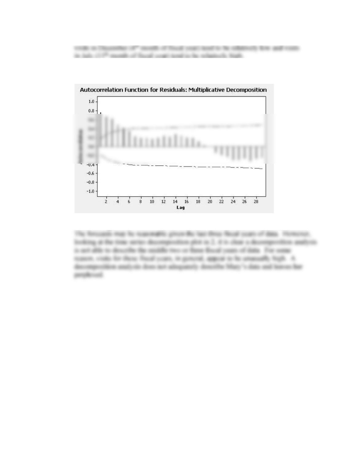
4. The residual autocorrelation function is shown below.
There are significant residual autocorrelations. The residuals are far from random