Chapter 5 Homework Data For Group Objects Made From The

Regression 1

5.8 Regression

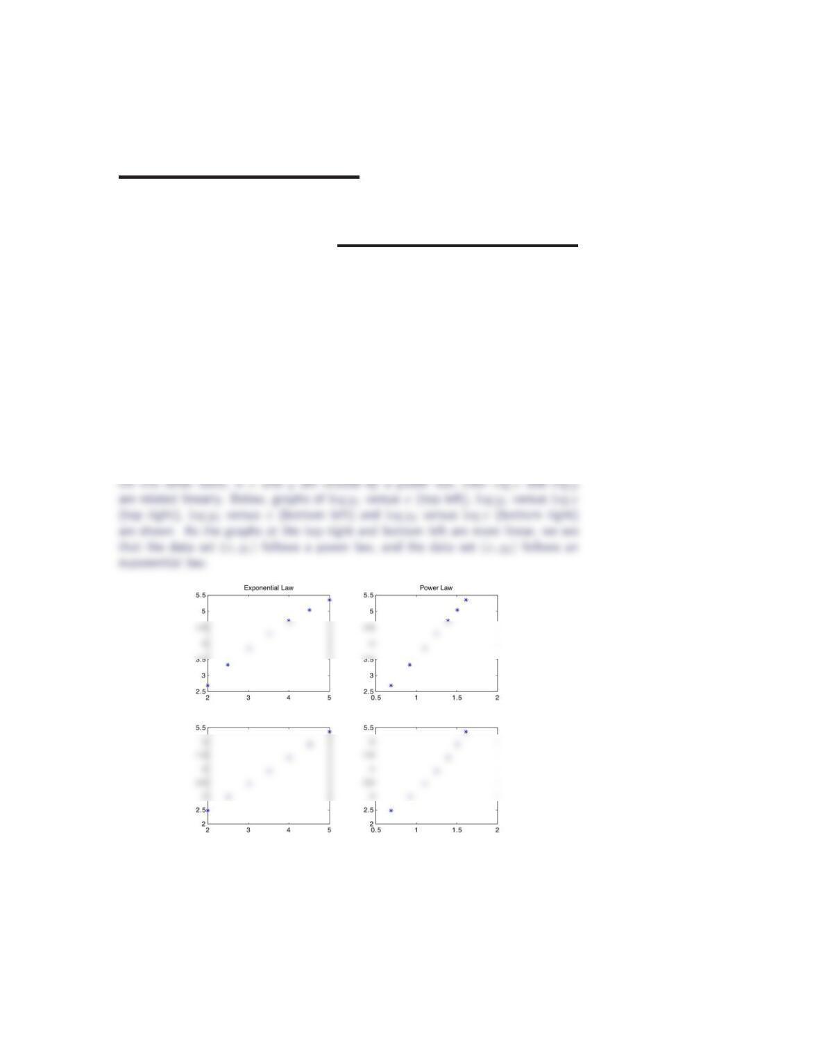
1. One of the following data sets follows an exponential law and the other follows

a power law. Which is which?

x2.0 2.5 3.0 3.5 4.0 4.5 5.0

y114.79 27.75 47.09 74.07 109.99 156.10 213.69

x2.0 2.5 3.0 3.5 4.0 4.5 5.0

y212.13 19.58 31.59 50.97 82.21 132.59 213.82

If xand yare related by an exponential law, then xand log yare linearly related.

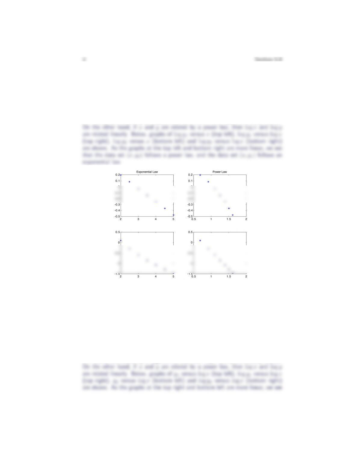
2. One of the following data sets follows an exponential law and the other follows

a power law. Which is which?

x2.0 2.5 3.0 3.5 4.0 4.5 5.0

y11.216 1.087 0.972 0.870 0.778 0.696 0.622

x2.0 2.5 3.0 3.5 4.0 4.5 5.0

y21.108 0.758 0.556 0.427 0.341 0.279 0.233

If xand yare related by an exponential law, then xand log yare linearly related.

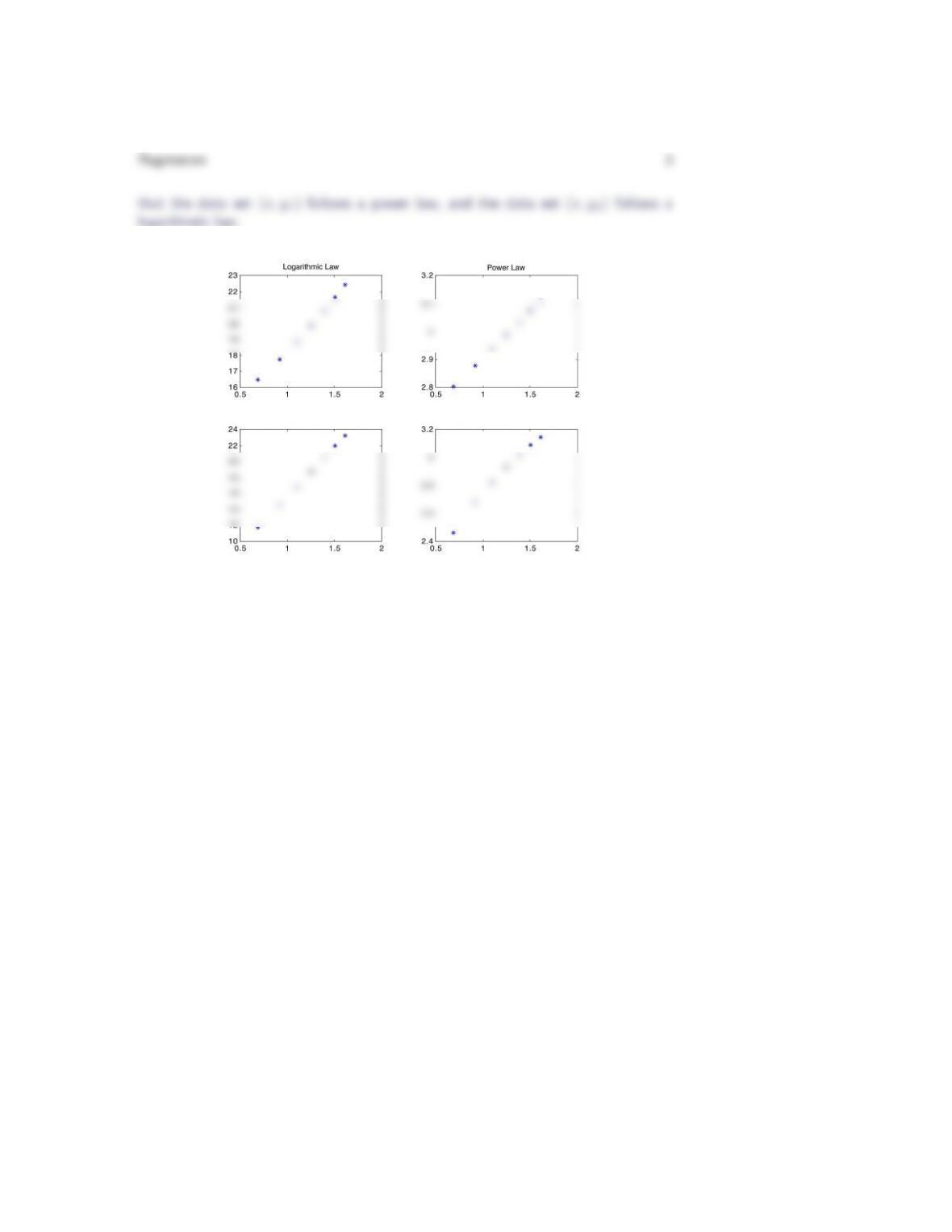
3. One of the following data sets follows a logarithmic law and the other follows a

power law. Which is which?

x2.0 2.5 3.0 3.5 4.0 4.5 5.0

y116.50 17.77 18.89 19.88 20.79 21.62 22.40

x2.0 2.5 3.0 3.5 4.0 4.5 5.0

y211.73 14.54 16.84 18.78 20.46 21.95 23.27

If xand yare related by a logarithmic law, then log xand yare linearly related.

4. Experimental data relating the oxide thickness, measured in Angstroms, of a

thin film to the baking time of the film, measured in minutes, is given in the

table below.

Baking Time 20 30 40 60 70 90 100 120 150 180

Oxide Thickness 3.5 7.4 7.1 15.6 11.1 14.9 23.5 27.1 22.1 32.9

(a) Construct a scatter plot of this data. What functional form is most appro-

priate for fitting this data?

(b) Fit the data to the function indicated in part (a). What physical signifi-

cance do the model parameters have?

(c) Predict the oxide thickness for a film which is baked for 45 minutes.

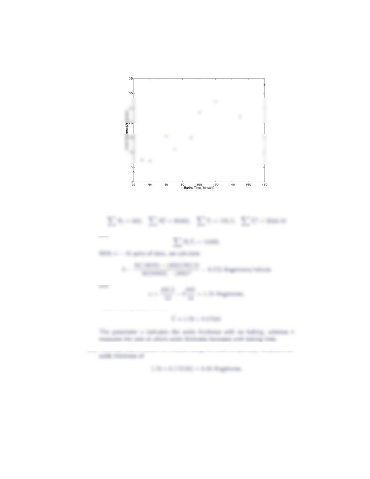
(a) A scatter plot of the data is given below. Based on this plot, it would be most

appropriate to fit the data to a linear function.

4Section 5.8

(b) Let Bidenote the baking time and Tithe oxide thickness of the i-th sample.

Then

Thus, the regression line is

(c) For a film that is baked 45 minutes, using the result of part (b), we predict an

5. The total production cost as a function of the number of machine hours is

provided for a sample of nine production runs. Estimate the fixed costs and the

variable costs associated with this process.

Regression 5

Machine Hours 22 23 19 12 12 9 7 11 14

Total Cost (in 1000’s) 23 25 20 20 20 15 14 14 16

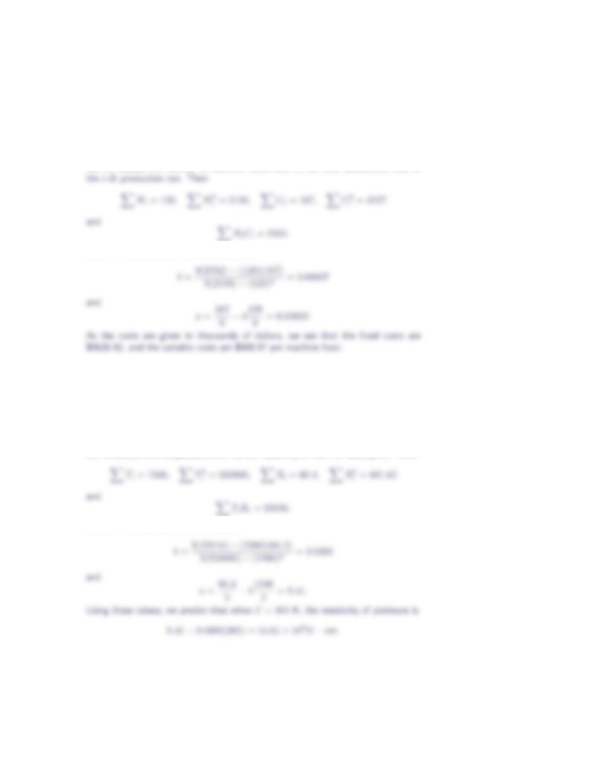
Let Hidenote the number of machine hours and Cithe total production cost of

With n= 9 production runs, we calculate

6. The resistivity of platinum as a function of temperature is given below. Estimate

the parameters in a linear fit to the data and predict the resistivity when the

temperature is 365 K.

Temperature (K) 100 200 300 400 500

Resistivity (Ω-cm, ×106) 4.1 8.0 12.6 16.3 19.4

Let Tidenote the temperature and Rithe resistivity of the i-th data point. Then

With n= 5 data points, we calculate

7. The table below shows the time (in seconds) required for water to drain through

a hole in the bottom of a bottle as a function of the depth (in inches) to which

the bottle has been filled.

Time 65.99 120.28 166.69 207.85 245.41 279.95 313.04 344.24

(a) Construct a scatter plot of this data. What functional form is most appro-

priate for fitting this data?

(b) Fit the data to the function indicated in part (a).

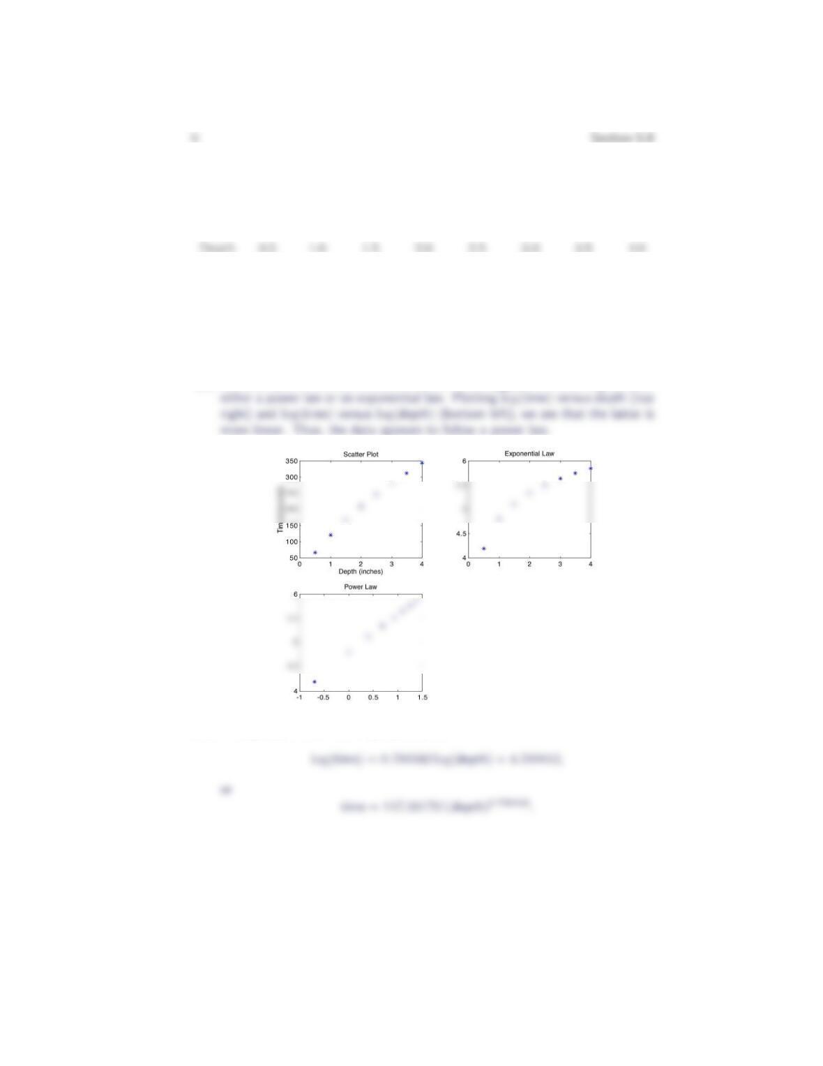
(a) A scatter plot of the data is shown below. This suggests the data might follow

(b) Fitting log(time)versus log(depth)yields

8. The weight, W, of a metallic object decreases over time when exposed to a

caustic environment according to the exponential law W=ae−t/τ , where tis

the exposure time and τis known as the decay rate constant. Data for a group

of objects made from the same material is given in the following table.

Regression 7

Exposure Time (days) 5 10 15 20 25 30 35 40

Weight (grams) 92.7 58.3 59.5 41.7 45.6 31.8 38.3 19.9

Estimate the decay rate constant, τ, for this material.

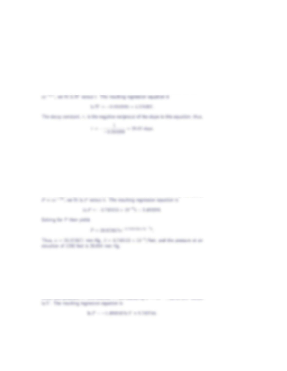
Given that weight, W, and exposure time, t, satisfy the exponential law W=

9. Barometric pressure, P, as a function of elevation above sea level, h, is modeled

by the relation P=αe−βh. Use the data in the table below to estimate the

model parameters and to predict the barometric pressure at an elevation of 1200

feet.

Barometric Pressure (mm Hg) 29.9 29.4 29.0 28.4 27.7

Elevation above Sea Level (feet) 0 500 1000 1500 2000

Given that pressure, P, and elevation above sea level, h, are related by the model

10. When an ideal gas undergoes an isentropic process, the pressure and volume

are related by P=cV −γ, where γis the ratio of the specific heats of the gas.

Estimate the value of γbased on the values in the following table:

Pressure (psi) 16.8 39.7 78.6 115.5 195.0 546.1

Volume (in3) 50 30 20 15 10 5

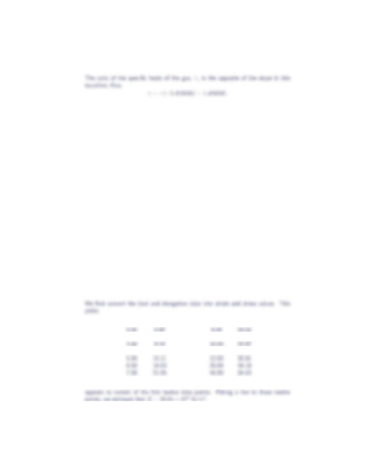
Given that pressure, P, and volume, V, are related by P=cV −γ, we fit ln Pversus

8Section 5.8

11. The results of a tensile strength test for a circular cold-rolled steel specimen are

provided in the table below. The specimen had an original diameter of 0.507”

and an original length of 2 inches. The normal stress, σ, and the normal strain,

ǫ, are given by the equations

σ=P

Aand ǫ=∆

L

where Pdenotes the load, ∆ the elongation, Athe original cross-sectional area

and Lthe original length of the specimen. From the test data, we want to

estimate the modulus of elasticity, E, which is defined as the ratio σ/ǫ in the

linear portion of the stress-strain curve.

load elongation load elongation

(103lbs) (10−4in) (103lbs) (10−4in)

0 0 4.85 16

1.25 4 5.45 18

1.85 6 6.05 20

2.4 8 6.7 22

3.05 10 7.25 24

3.64 12 6.9 40

4.25 14 6.95 80

NOTE: For this problem, you will first need to decide which of the data points

correspond to the linear portion of the stress-strain curve.

ǫ×10−4σ×103ǫ×10−4σ×103

2.00 6.19 9.00 27.00

4.00 11.89 11.00 33.19

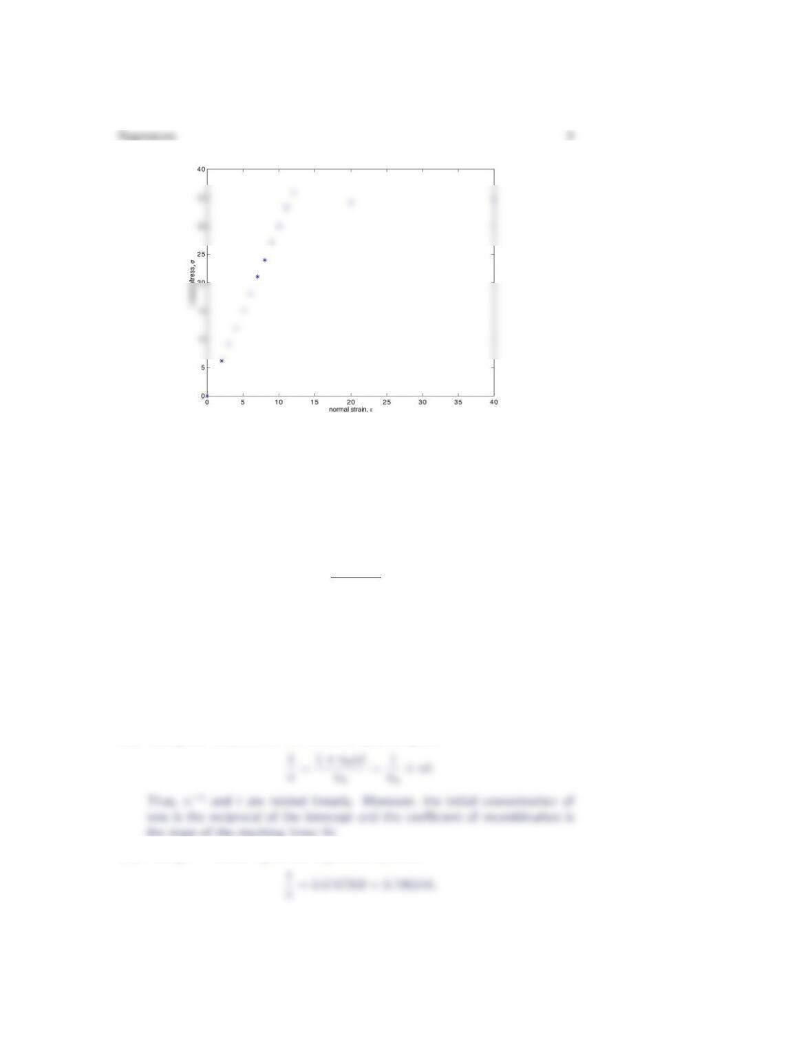
A plot of the stress-strain curve is shown below. The linear portion of the curve

12. The following table gives the ion concentration, n, as a function of time, t, after

an ionization agent has been turned oﬀ.

time (sec) 0 1 2 3 4 5 6 7 8 9 10

n(×10−4) 5.03 4.71 4.40 3.97 3.88 3.62 3.30 3.15 3.08 2.92 2.70

Theory indicates that ion concentration and time satisfy the reciprocal relation-

ship

n=n0

1 + n0αt,

where n0is the initial concentration of ions and αis the coefficient of recombi-

nation.

(a) Take the reciprocal of the above equation relating ion concentration and

time, and show that n−1and tare related in a linear fashion.

(b) Perform linear regression on n−1versus tto estimate the initial concentra-

tion of ions and the coefficient of recombination.

(a) Taking the reciprocal of the indicated equation gives

the slope of the resulting linear fit.

(b) Fitting n−1versus tgives the regression equation

10 Section 5.8

Thus, we estimate that

13. Consider the following data relating the amount of varnish additive and the

resulting varnish drying time.

additive (grams) 0.0 1.0 2.0 3.0 4.0 5.0 6.0 7.0 8.0

drying time (hours) 12.0 10.5 10.0 8.0 7.0 8.0 7.5 8.5 9.0

(a) Produce a scatter plot of the data and show that the data roughly follows

the pattern of a quadratic function.

(b) Apply the least-squares criterion to the regression equation ˆy=a+bx+cx2

to determine formulas for a,band c.

(c) Use the results of part (b) to determine the regression parabola for the data

given above. What amount of varnish additive will produce the minimum

drying time?

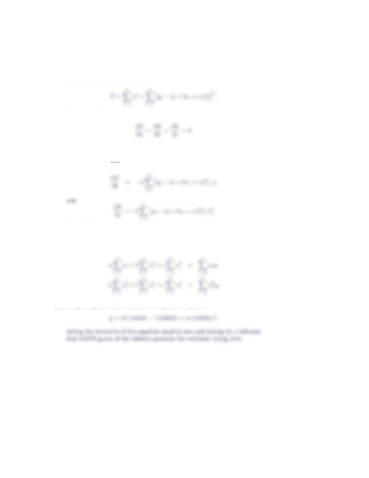
(a) The scatter plot shown below has the rough shape of an upward opening

parabola.

(b) Let (xi, yi)denote the data pairs being examined, and let eimeasure the

Regression 11

Denote the total error, E, by

To minimize E, we must have

Because

∂E

∂a =−2

n

X

i=1

yi−(a+bxi+cx2

i)

the coefficients a,band csatisfy the system

na +b

n

X

i=1

xi+c

n

X

i=1

x2

i=

n

X

i=1

yi

(c) Using the given data, we obtain the regression equation