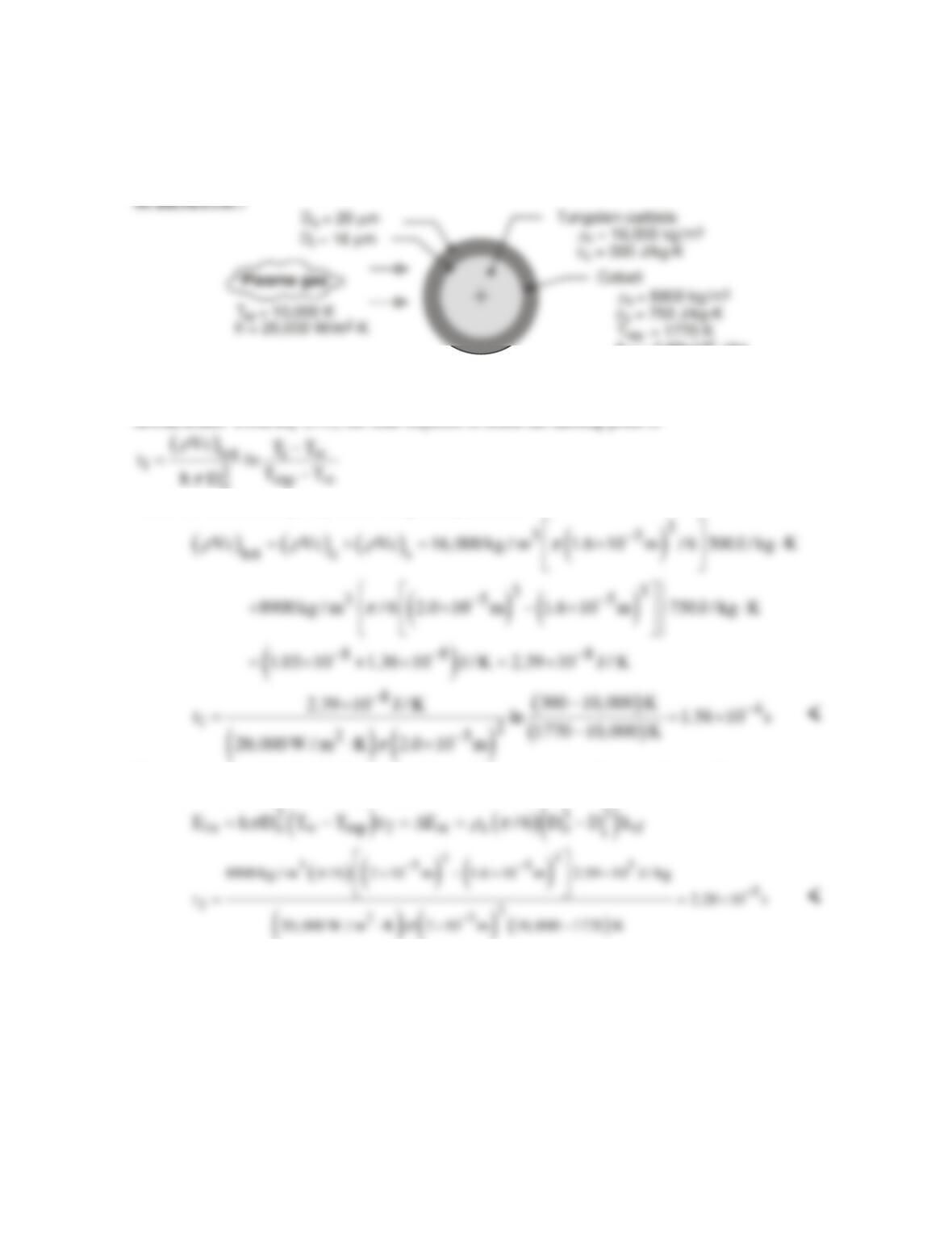
PROBLEM 5.30
KNOWN: Diameters, initial temperature and thermophysical properties of WC and Co in composite
particle. Convection coefficient and freestream temperature of plasma gas. Melting point and latent
heat of fusion of Co.
FIND: Times required to reach melting and to achieve complete melting of Co.
sf 5
h = 2.59×10 J/kg
ASSUMPTIONS: (1) Particle is isothermal at any instant, (2) Radiation exchange with surroundings
is negligible, (3) Negligible contact resistance at interface between WC and Co, (4) Constant
properties.
ANALYSIS: From Eq. (5.5), the time required to reach the melting point is
o
where the total heat capacity of the composite particle is
The time required to melt the Co may be obtained by applying the first law, Eq. (1.12b) to a control
surface about the particle. It follows that
COMMENTS: (1) The largest value of the radiation coefficient corresponds to hr = εs (Tmp + Tsur)
( )
22
mp sur
T T.+
For the maximum possible value of ε = 1 and Tsur = 300K, hr = 378 W/m2⋅K << h =
20,000 W/m2⋅K. Hence, the assumption of negligible radiation exchange is excellent. (2) Despite the
large value of h, the small values of Do and Di and the large thermal conductivities (~ 40 W/m⋅K and
70 W/m⋅K for WC and Co, respectively) render the lumped capacitance approximation a good one.
(3) A detailed treatment of plasma heating of a composite powder particle is provided by Demetriou,
Lavine and Ghoniem (Proc. 5th ASME/JSME Joint Thermal Engineering Conf., March, 1999).
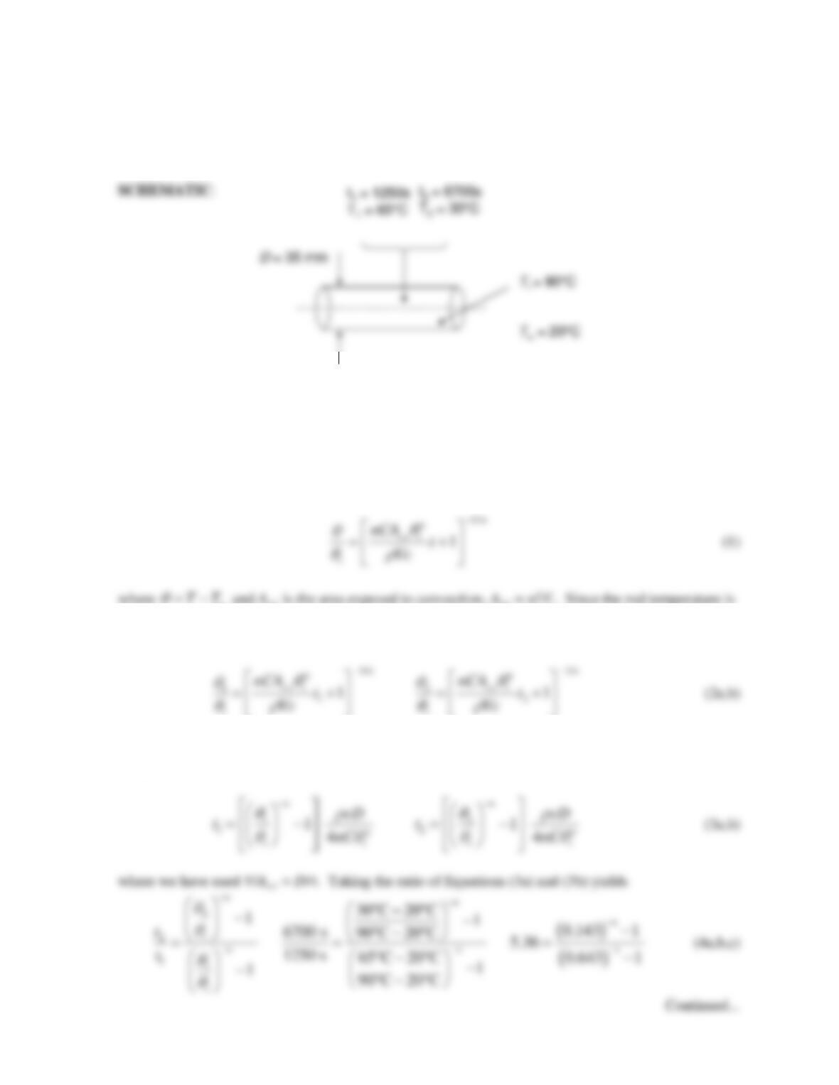
PROBLEM 5.31
KNOWN: Diameter of highly polished aluminum rod. Temperature of rod initially and at two later
times. Room air temperature.
FIND: Values of constants C and n in Equation 5.26. Plot rod temperature vs. time for varying and
constant heat transfer coefficients.
ASSUMPTIONS: (1) Constant properties, (2) Radiation negligible because rod is highly polished,
(3) Lumped capacitance approximation is valid.
PROPERTIES: Table A.1, Aluminum (T = 328 K): c = 916 J/kg⋅K,
ρ
= 2702 kg/m3, k = 238
W/m⋅K.
ANALYSIS: If the heat transfer coefficient is given by Equation 5.26, then the temperature as a
function of time is given by Equation 5.28:
∞
known at two different times, Equation (1) can be evaluated at these two times, making it possible to
solve for the two unknowns, C and n. The two equations are
These equations cannot be explicitly solved for C and n. They can be numerically solved in this form,
using IHT or some other software, or they can be further manipulated to solve for the times:
PROBLEM 5.31 (Cont.)
This can be iteratively or numerical solved for n, to find n = 0.25. Then C can be determined from
Equation (3a) or (3b):
Now that these constants are known, the validity of the lumped capacitance approximation can
checked. The maximum heat transfer coefficient occurs at the initial time,
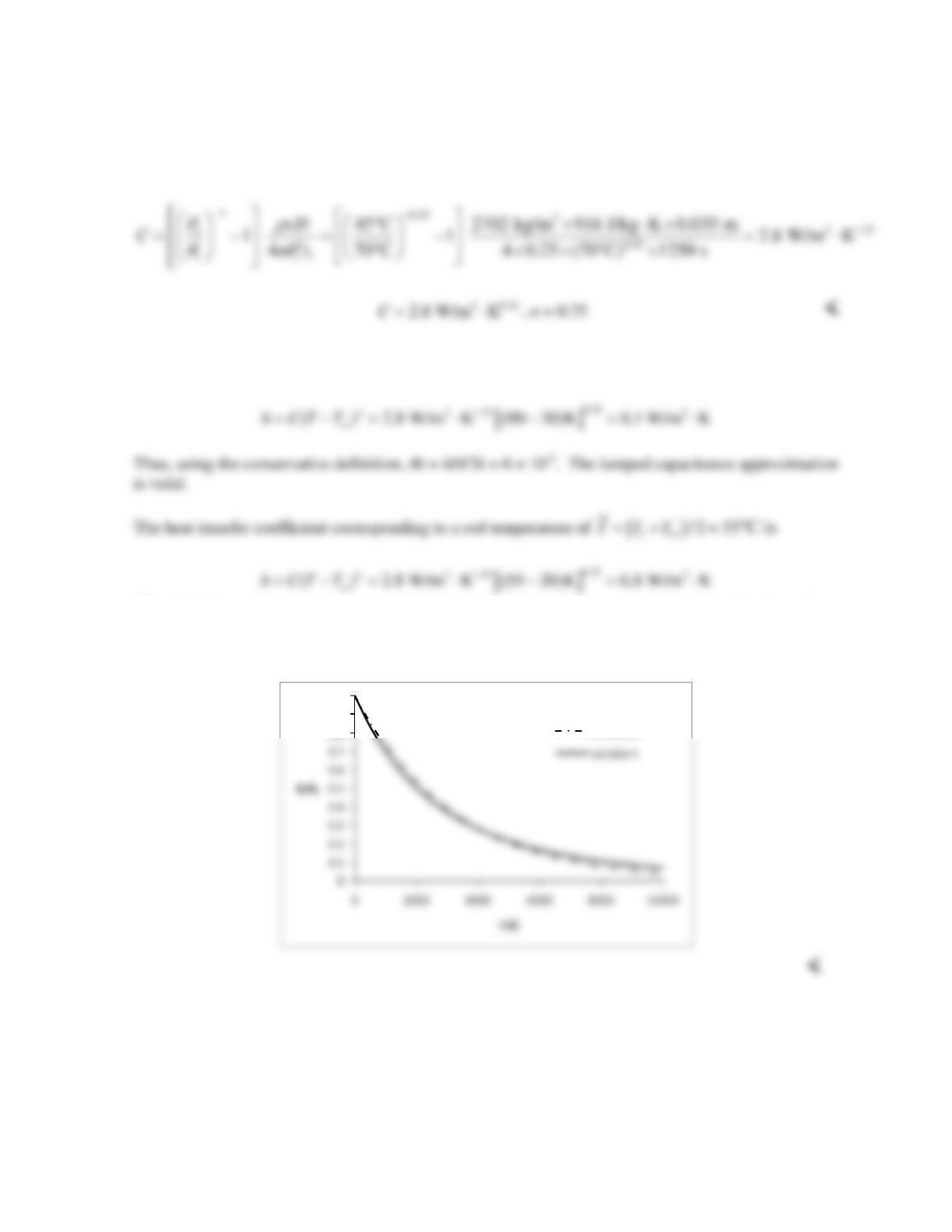
The plot below shows the rod temperature as a function of time using Equation (1) above for
variable heat transfer coefficient, as well as the rod temperature assuming the constant value
of h = 6.8 W/m2⋅K, using text Equation 5.6.
0.8
0.9
1
constant h
COMMENTS: (1) Since the heat transfer coefficient is temperature difference-dependent (variable
h), the initial cooling rates are larger when this dependence is accounted for. As the temperature
difference decreases, the variable h case cools slower relative to the constant h case. (2) The
discrepancy between the variable and constant heat transfer coefficient cases is not large under these
conditions. The difference would be greater if n were larger.
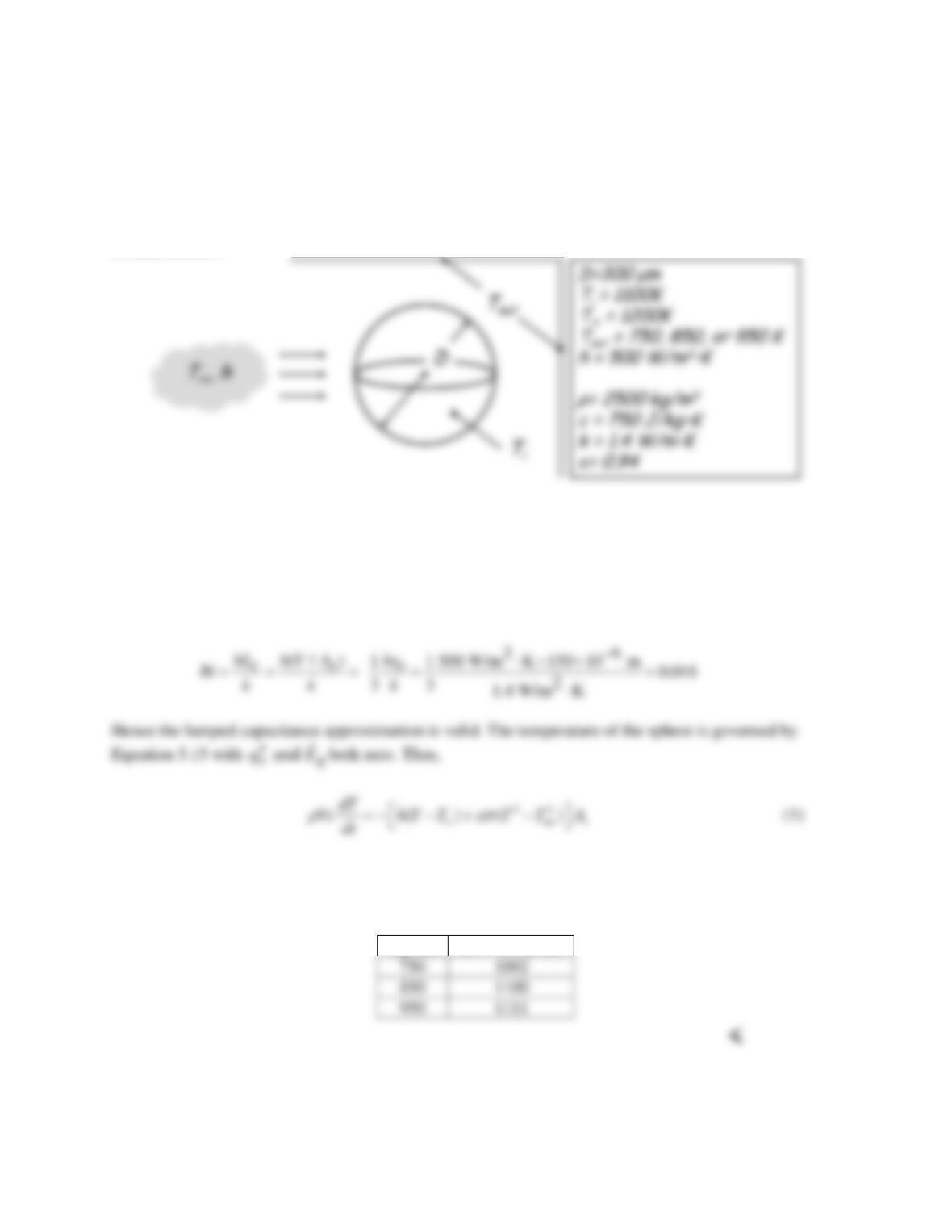
PROBLEM 5.32
KNOWN: Spherical ceramic particle of known properties, diameter, and initial temperature.
Environment temperature and heat transfer coefficient.
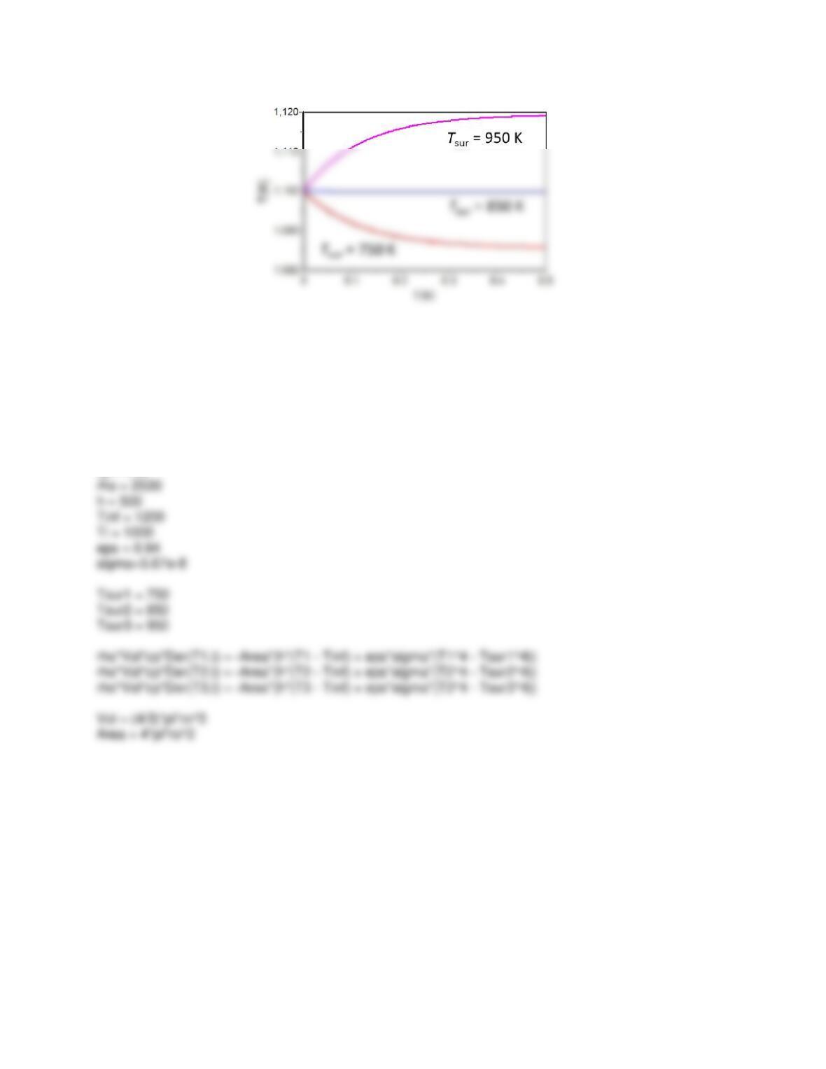
FIND: Particle temperature at t = 0.1 s for Tsur = 750 K, 850 K, and 950 K. Plot of particle temperature
vs. time.
SCHEMATIC:
ASSUMPTIONS: (1) Radiation can be approximated as a small object in large surroundings, (2)
Uniform properties, (3) The lumped capacitance approximation is valid.
PROPERTIES: Given,
ρ
= 2500 kg/m3, cp =750 J/kg⋅K, k = 1.4 W/m⋅K,
ε
= 0.94.
ANALYSIS: The Biot number is
This differential equation can be solved numerically subject to the initial condition T(t = 0) = Ti = 1100 K.
Using the Der function of IHT (see code in Comments section), the particle temperature at t = 0.1 s for
the three surroundings temperatures of 750, 850, and 950 K are:
Tsur (K)
T(t = 0.1 s) (K)
The particle temperature as a function of time is shown below for the three surroundings temperatures.
Continued…
PROBLEM 5.32 (Cont.)
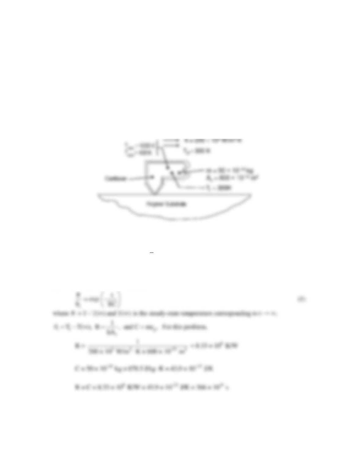
COMMENTS: (1) The IHT code is given below. (2) Depending on the surroundings temperature, the
particle temperature can decrease, stay the same, or increase. (3) The steady–state temperature can be
found by setting dT/dt = 0 in Eq. (1) and solving for Tss. The results for the three surroundings
temperatures are Tss = 1086, 1100, and 1119 K for Tsur = 750, 850, and 950 K, respectively.
D = 300e-6
ro = D/2
k = 1.4
cp = 750
PROBLEM 5.33
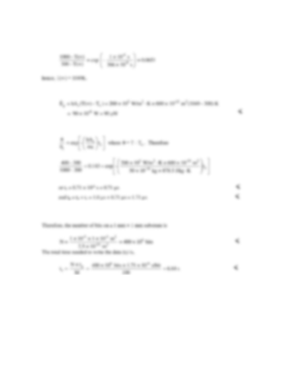
KNOWN: Mass and exposed surface area of a silicon cantilever, convection heat transfer
coefficient, initial and ambient temperatures.
FIND: (a) The ohmic heating needed to raise the cantilever temperature from Ti = 300 K to T =
1000 K in th = 1
s, (b) The time required to cool the cantilever from T = 1000 K to T = 400 K, tc
and the thermal processing time (tp = th + tc), (c) The number of bits that can be written onto a 1
mm 1 mm surface area and time needed to write the data for a processing head equipped with
M cantilevers.
SCHEMATIC:
ASSUMPTIONS: (1) Lumped capacitance behavior, (2) Negligible radiation heat transfer, (3)
Constant properties, (4) Negligible heat transfer to polymer substrate.
PROPERTIES: Table A.1, silicon (
T
= 650 K): cp = 878.5 J/kgK.
ANALYSIS:
(a) From Problem 5.17 we note that
Therefore, Equation 1 may be evaluated as
Continued…
PROBLEM 5.33 (Cont.)
At steady-state, Equation 1.12b yields
(b) Equation 5.6 may be used. Hence,
(c) Each bit occupies Ab = 50 × 10-9 m × 50 × 10-9 m = 2.5 × 10⁻¹⁵ m2
COMMENTS: (1) Lumped thermal capacitance behavior is an excellent approximation for such
a small device (2) Each cantilever writes N/M = 400 106 bits/100 cantilevers = 400 104
bits/cantilever. With a separation distance of 50 10-9 m, the total distance traveled is 50 10-9 m
400 104 = 200 10-3 m = 200 mm. If the head travels at 200 mm/s, it will take 1 second to
move the head, providing a total writing and moving time of 6.84 s + 1 s = 7.84 s. The speed of
the process is heat transfer-limited.
PROBLEM 5.34
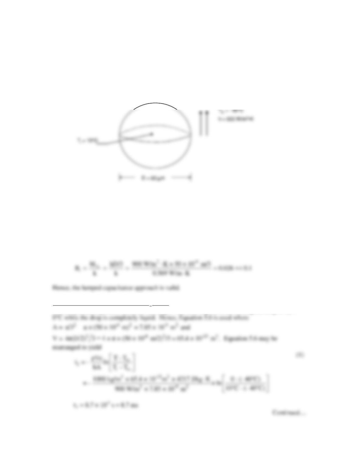
KNOWN: Ambient conditions, initial water droplet temperature and diameter.
FIND: Total time to completely freeze the water droplet for (a) droplet solidification at Tf = 0°C
and (b) rapid solidification of the droplet at Tf,sc .
SCHEMATIC:
ASSUMPTIONS: (1) Isothermal particle, (2) Negligible radiation heat transfer, (3) Constant
properties.
PROPERTIES: Table A.6, liquid water (T = 0 °C): cp = 4217 J/kg⋅K, k = 0.569 W/m⋅K, ρ =
1000 kg/m3. Example 1.5: hsf = 334 kJ/kg.
ANALYSIS: We begin by evaluating the validity of the lumped capacitance method by
determining the value of the Biot number.
Case A: Equilibrium solidification, Tf = 0°C.
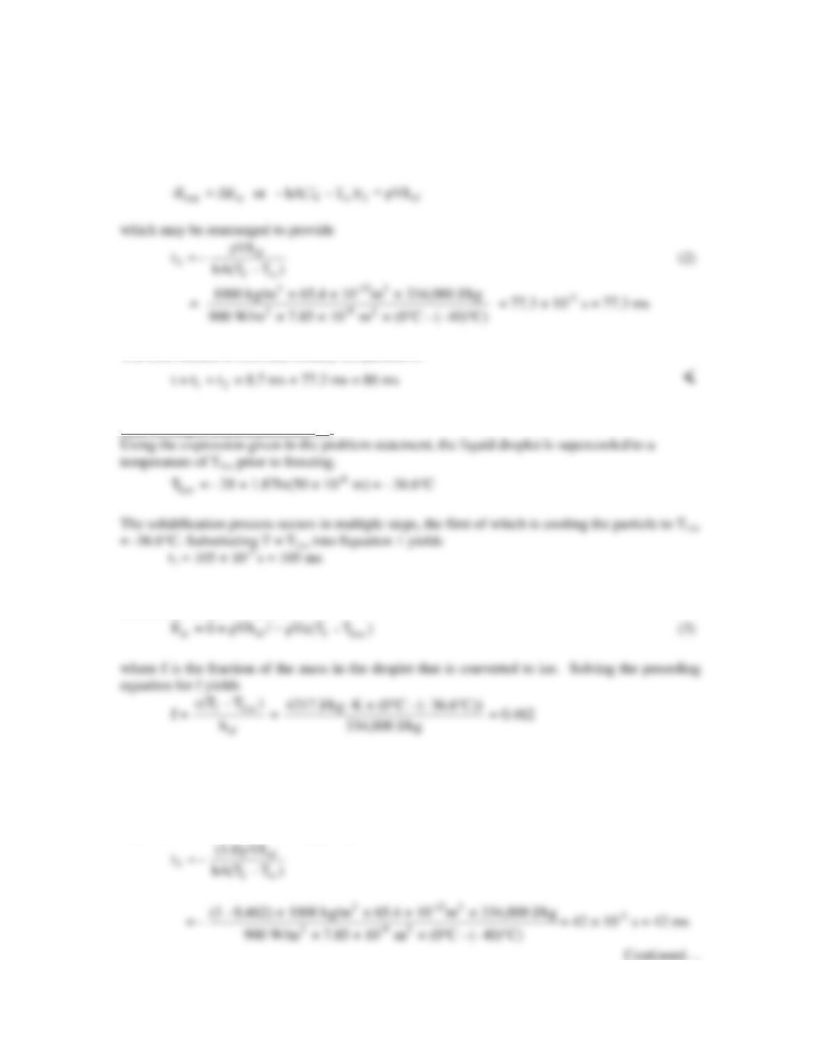
The solidification process occurs in two steps. The first step involves cooling the drop to Tf =
PROBLEM 5.34 (Cont.)
The second step involves solidification of the ice, which occurs at Tf = 0°C. An energy balance
on the droplet yields
The time needed to cool and solidify the particle is
Case B: Rapid solidification at Tf,sc .
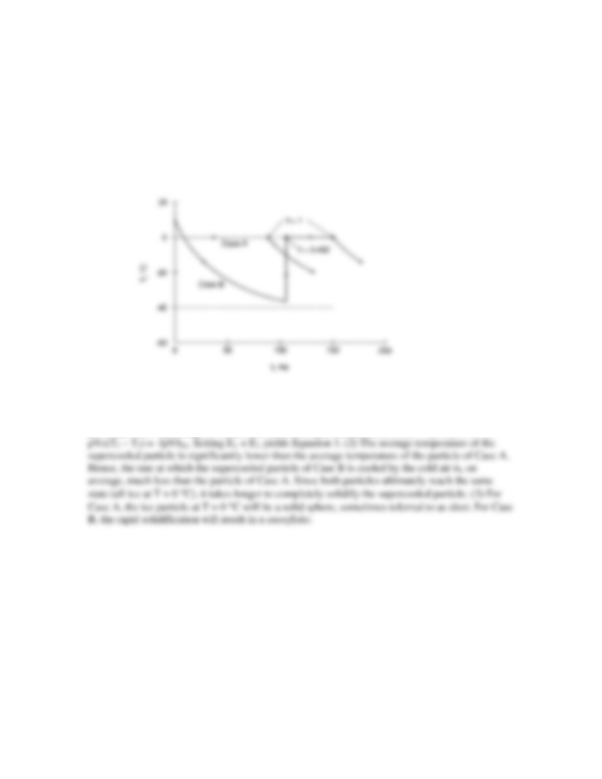
The second step involves rapid solidification of some or all of the supercooled liquid. An energy
balance on the particle yields
Hence, immediately after the rapid solidification, the water droplet is approximately 46% ice and
54% liquid. The time required for the rapid solidification is t2 ≈ 0 s.
The third stage of Case B involves the time required to freeze the remaining liquid water, t3.
Equation 2 is modified accordingly to yield
PROBLEM 5.34 (Cont.)
The total time to solidify the particle is
t = t1 + t2 + t3 = 105 ms + 0 + 42 s = 147 ms <
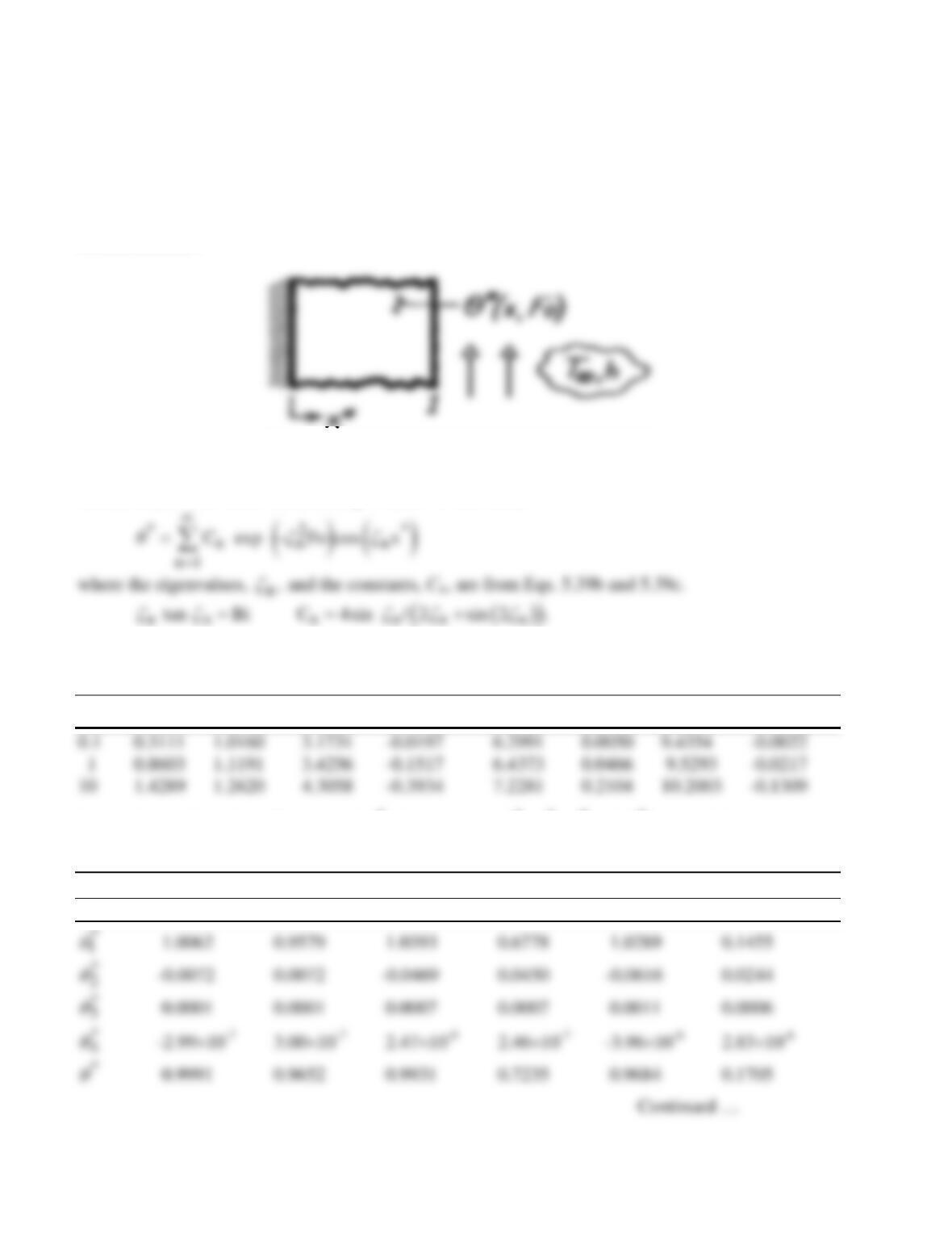
The temperature histories associated with Case A and Case B are shown in the sketch below.
COMMENTS: (1) Equation 3 may be derived by assuming a reference temperature of Tf = 0 °C
and a liquid reference state. The energy of the particle prior to the rapid solidification is E1 =
ρVc(Tf,sc – Tf). The energy of the particle after the rapid solidification is E2 = -fρVhsf + (1 – f)
PROBLEM 5.35
KNOWN: Series solution, Eq. 5.42, for transient conduction in a plane wall with convection.
FIND: Midplane (x*=0) and surface (x*=1) temperatures θ* for Fo=0.1 and 1, using Bi=0.1, 1 and
10 with only the first four eigenvalues. Based upon these results, discuss the validity of the
approximate solutions, Eqs. 5.43 and 5.44.
SCHEMATIC:
ASSUMPTIONS: (1) One-dimensional transient conduction, (2) Constant properties.
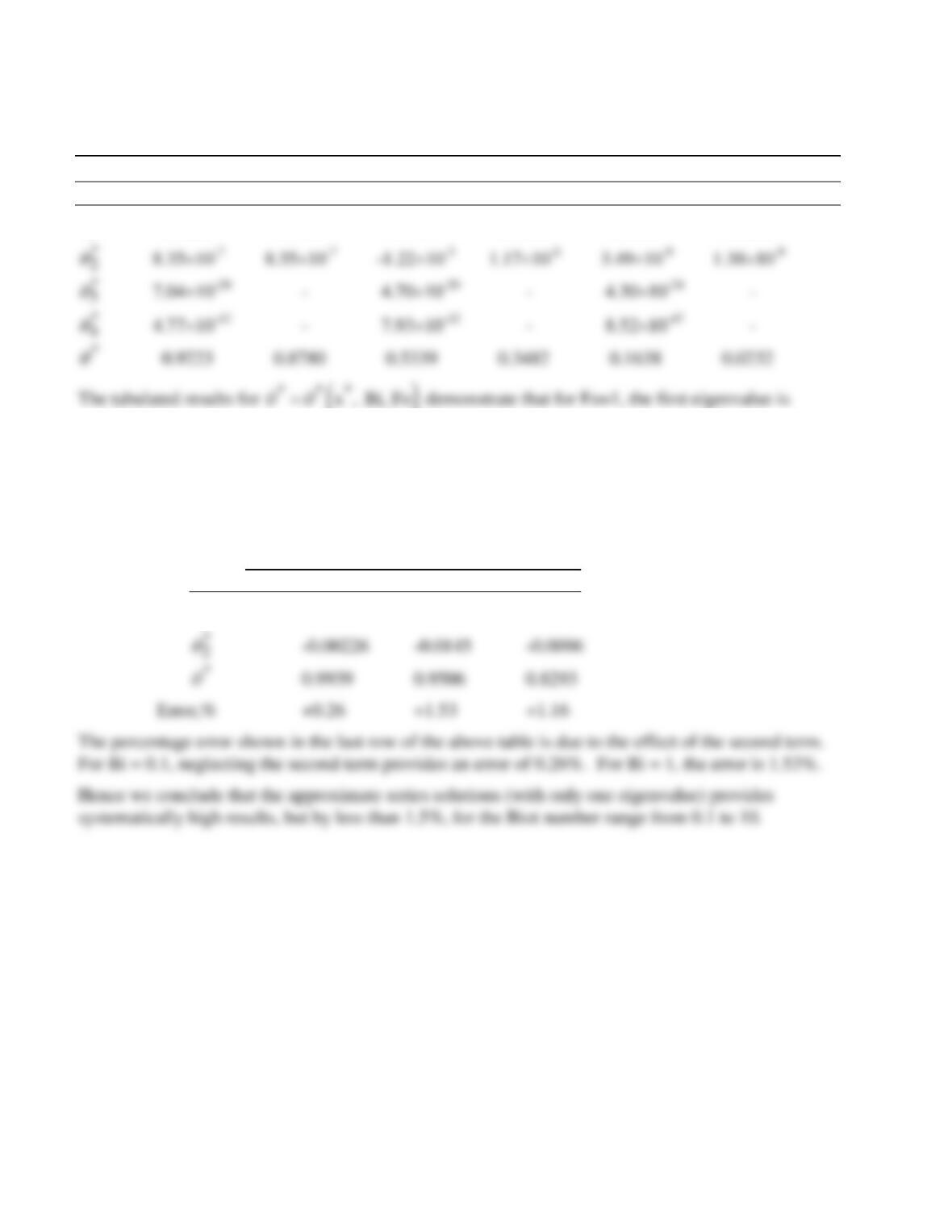
ANALYSIS: The series solution, Eq. 5.42a, is of the form,
The eigenvalues are tabulated in Appendix B.3; note, however, that
1
ζ
and C1 are available from
Table 5.1. The values of
n
ζ
and Cn used to evaluate θ* are as follows:
Bi
1
ζ
C1
2
ζ
C2
3
ζ
C3
4
ζ
C4
Using
n
ζ
and Cn values, the terms of
*
θ
, designated as
*** *
1 23 4
, , and ,
θθθ θ
are as follows:
Fo=0.1
Bi=0.1 Bi=1.0 Bi=10
x* 0 1 0 1 0 1
PROBLEM 5.35 (Cont.)
Fo=1
Bi=0.1 Bi=1.0 Bi=10
x* 0 1 0 1 0 1
*
1
θ
0.9223 0.8780 0.5339 0.3482 0.1638 0.0232
()
sufficient to accurately represent the series. However, for Fo=0.1, three eigenvalues are required for
accurate representation.
A more detailed analysis would show that a practical criterion for representation of the series solution
by one eigenvalue is Fo > 0.2. For these situations the approximate solutions, Eqs. 5.43 and 5.44, are
appropriate. For the midplane, x*=0, the first two eigenvalues for Fo=0.2 are:
Fo=0.2 x*=0
Bi 0.1 1.0 10
*
1
θ
0.9965 0.9651 0.8389
*
θ
*
θ
*
θ
PROBLEM 5.36
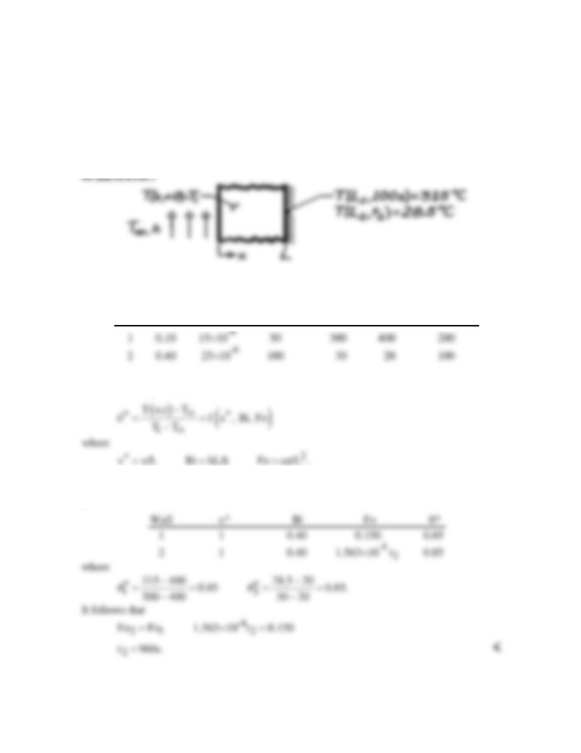
KNOWN: One–dimensional wall, initially at a uniform temperature, Ti, is suddenly exposed
to a convection process (T∞, h). For wall #1, the time (t1 = 100s) required to reach a
specified temperature at x = L is prescribed, T(L1, t1) = 315°C.
FIND: For wall #2 of different thickness and thermal conditions, the time, t2, required for
T(L2, t2) = 28°C.
ASSUMPTIONS: (1) One-dimensional conduction, (2) Constant properties.
ANALYSIS: The properties, thickness and thermal conditions for the two walls are:
Wall L(m) α(m2/s) k(W/m⋅K) Ti(°C) T∞(°C) h(W/m2⋅K)
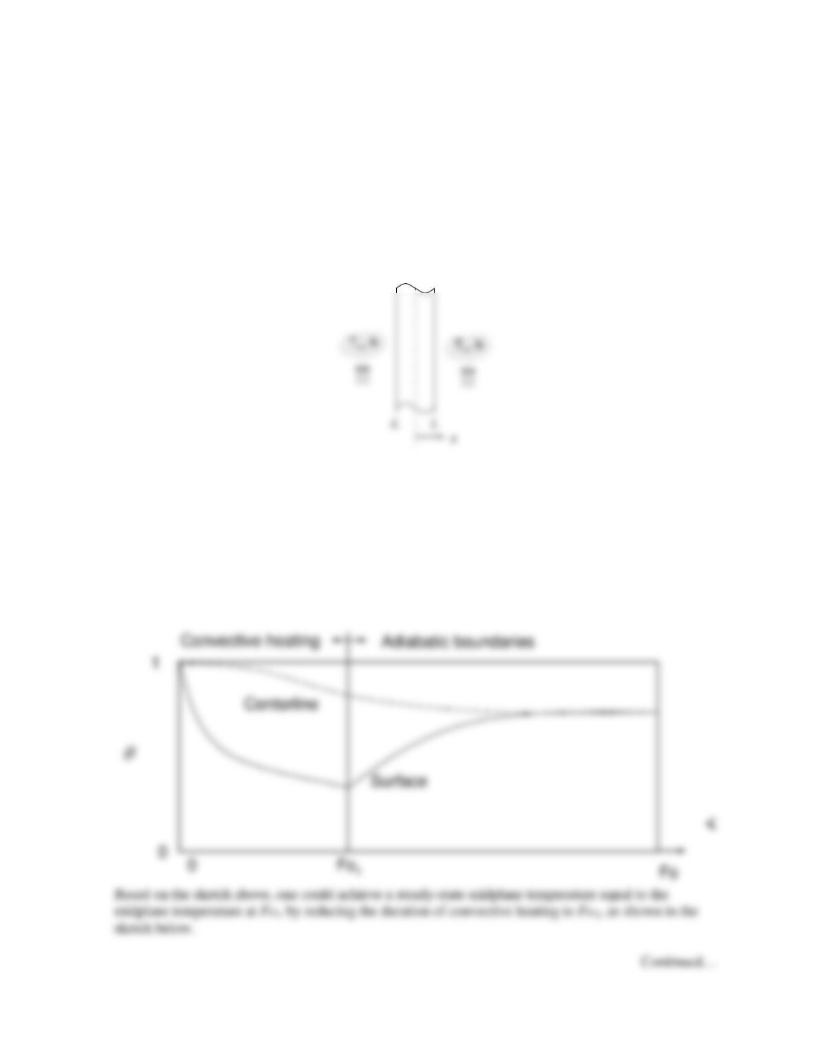
The dimensionless functional dependence for the one-dimensional, transient temperature
distribution, Eq. 5.38, is
If the parameters x*, Bi, and Fo are the same for both walls, then
12
.
θθ
∗∗
=
Evaluate these
parameters:
PROBLEM 5.37
KNOWN: One–dimensional convective heating of a plane slab with Bi = 1 for a dimensionless time
of Fo1.
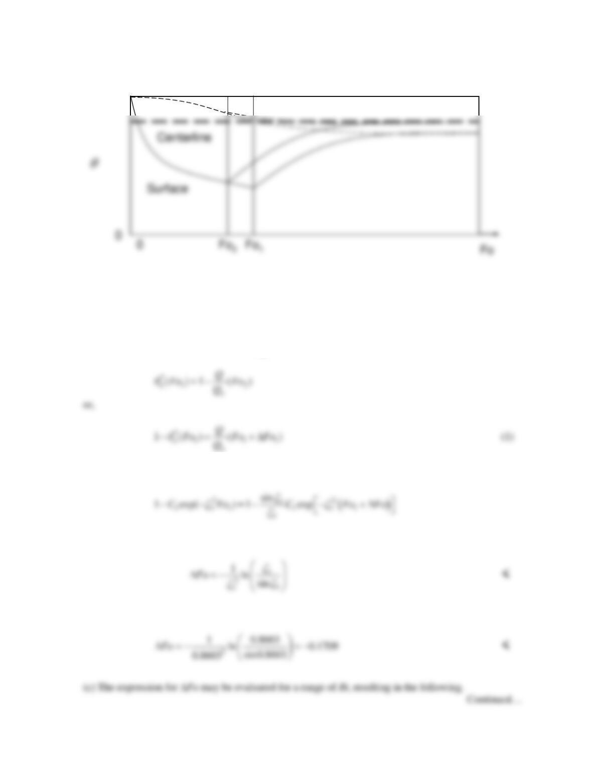
FIND: (a) Sketch of the dimensionless midplane and surface temperatures of the slab as a function of
dimensionless time over the range 0 < Fo1 < Fo < ∞. Relative value of Fo2, needed to achieve a
steady–state midplane temperature equal to the midplane temperature at Fo1. (b) Analytical expression
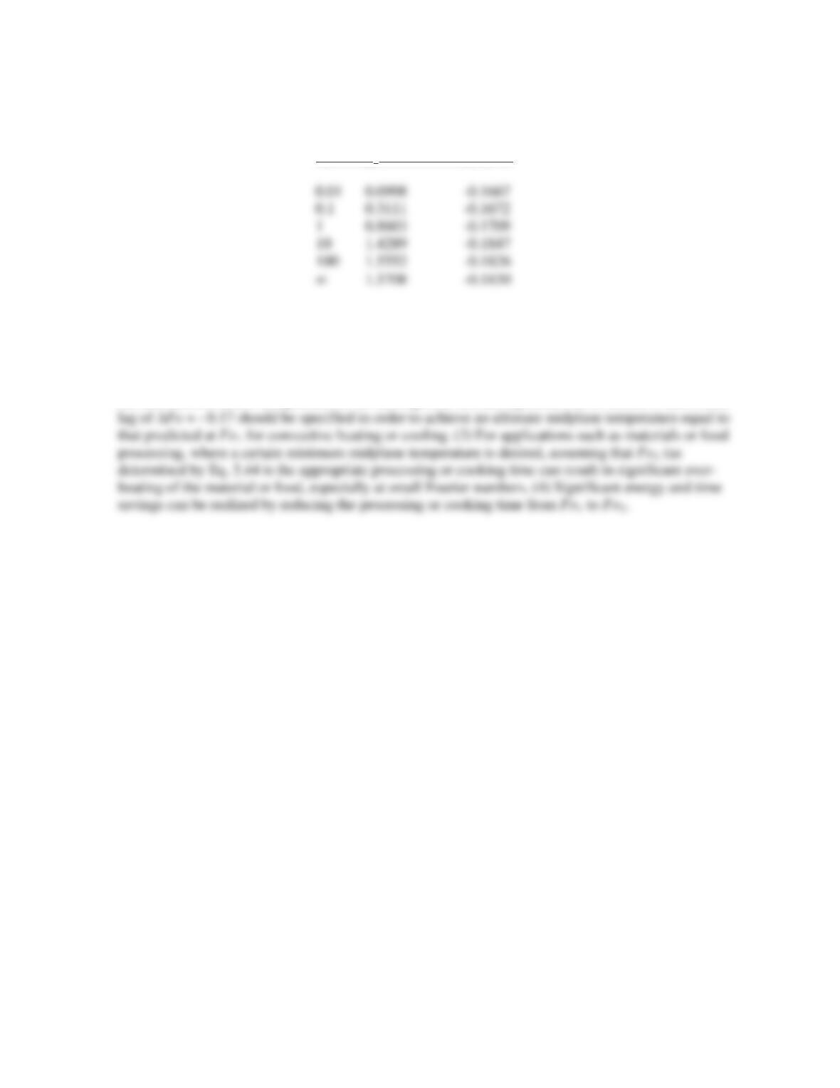
for, and value of ∆Fo = Fo2 – Fo1 for Bi = 1, Fo1 > 0.2, Fo2 > 0.2. (c) Value of ∆Fo for Bi = 0.01, 0.1,
10, 100 and ∞.
SCHEMATIC:
ASSUMPTIONS: (1) One–dimensional conduction, (2) Constant properties, (3) Approximate, one-
term solutions are valid.
ANALYSIS: (a) A sketch of the dimensionless midplane and surface temperatures is shown below.
Note that, at Fo1, the surface of the slab will be warm (small
θ
) relative to the midplane since
temperature gradients within the slab are significant (Bi = 1). At the curtailment of heating (Fo1), the
surface temperature cools rapidly while warm temperatures continue to propagate toward the
midplane, slowly heating the midplane until a steady-state, isothermal condition is eventually reached.
PROBLEM 5.37 (Cont.)
Hence, Fo2 < Fo1. <
(b) Using the approximate solutions of Section 5.5.2, and noting that the steady-state temperature of
the slab is uniform and related to the energy transferred to the slab,
Substituting Eqs. 5.44 and 5.49 into Eq. (1) yields
which may be simplified to
From Table 5.1,
ζ
1 = 0.8603 rad at Bi = 1. Hence,
1
PROBLEM 5.37 (Cont.)
Bi
ζ
1 ∆Fo <
COMMENTS: (1) Note that the dimensionless temperature,
( )
*2
11
exp
o
C Fo
θζ
= −
, is defined in a
manner such that for slab heating, increases in actual temperature correspond to decreases in the
dimensionless temperature. (2) The dimensionless time lag, ∆Fo, is weakly-dependent on the value of
the Biot number and is independent of the heating time. Hence, a general rule-of-thumb is that a time
PROBLEM 5.38
KNOWN: Thickness, properties and initial temperature of steel slab. Convection conditions.
FIND: Heating time required to achieve a minimum temperature of 550°C in the slab.
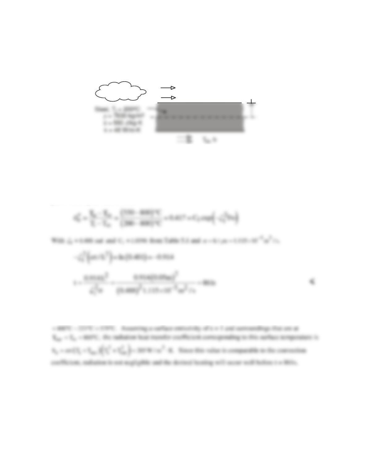
SCHEMATIC:
L = 0.05 m
T = 800
o
C
o
o
h = 250 W/m -K
2
Combustion
gases
ASSUMPTIONS: (1) One-dimensional conduction, (2) Negligible radiation effects, (3) Constant
properties.
ANALYSIS: With a Biot number of hL/k = (250 W/m2⋅K × 0.05m)/48 W/m⋅K = 0.260, a lumped
capacitance analysis should not be performed. At any time during heating, the lowest temperature in
the slab is at the midplane, and from the one-term approximation to the transient thermal response of a
plane wall, Eq. (5.44), we obtain
COMMENTS: The surface temperature at t = 861s may be obtained from Eq. (5.43b), where
( )
( )
o1
cos 0.417 cos 0.488 rad 0.368.x
θθ ζ
∗∗ ∗
= = =
Hence,
( ) ( )
si
T L, 861s T T 0.368 T T
∞∞
≡= + −
PROBLEM 5.39
KNOWN: Thickness and initial temperature of acrylic sheet.
FIND: Time needed to bring the external surface of the acrylic to its softening temperature.
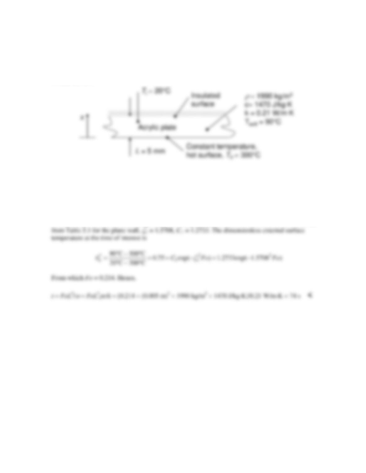
SCHEMATIC:
ASSUMPTIONS: (1) One–dimensional conduction, (2) Constant properties, (3) One-term
approximate solution is valid.
PROPERTIES: Acrylic (given):
ρ
= 1990 kg/m3, c = 1470 J/kg⋅K and k = 0.21 W/m⋅K.
ANALYSIS: For the constant temperature boundary condition, the Biot number is Bi → ∞. Hence,
COMMENTS: (1) Since Fo = 0.214 is greater than 0.2, the one-term approximation is valid. (2) A
contact resistance would be present at the interface between the acrylic and the substrate. However, as
the acrylic softens and deforms locally to make better contact with the substrate, the thermal contact
resistance would decrease in value.
PROBLEM 5.40
KNOWN: Thickness, initial temperature and properties of furnace wall. Convection conditions at
inner surface.
FIND: Time required for outer surface to reach a prescribed temperature. Corresponding
temperature distribution in wall and at intermediate times.
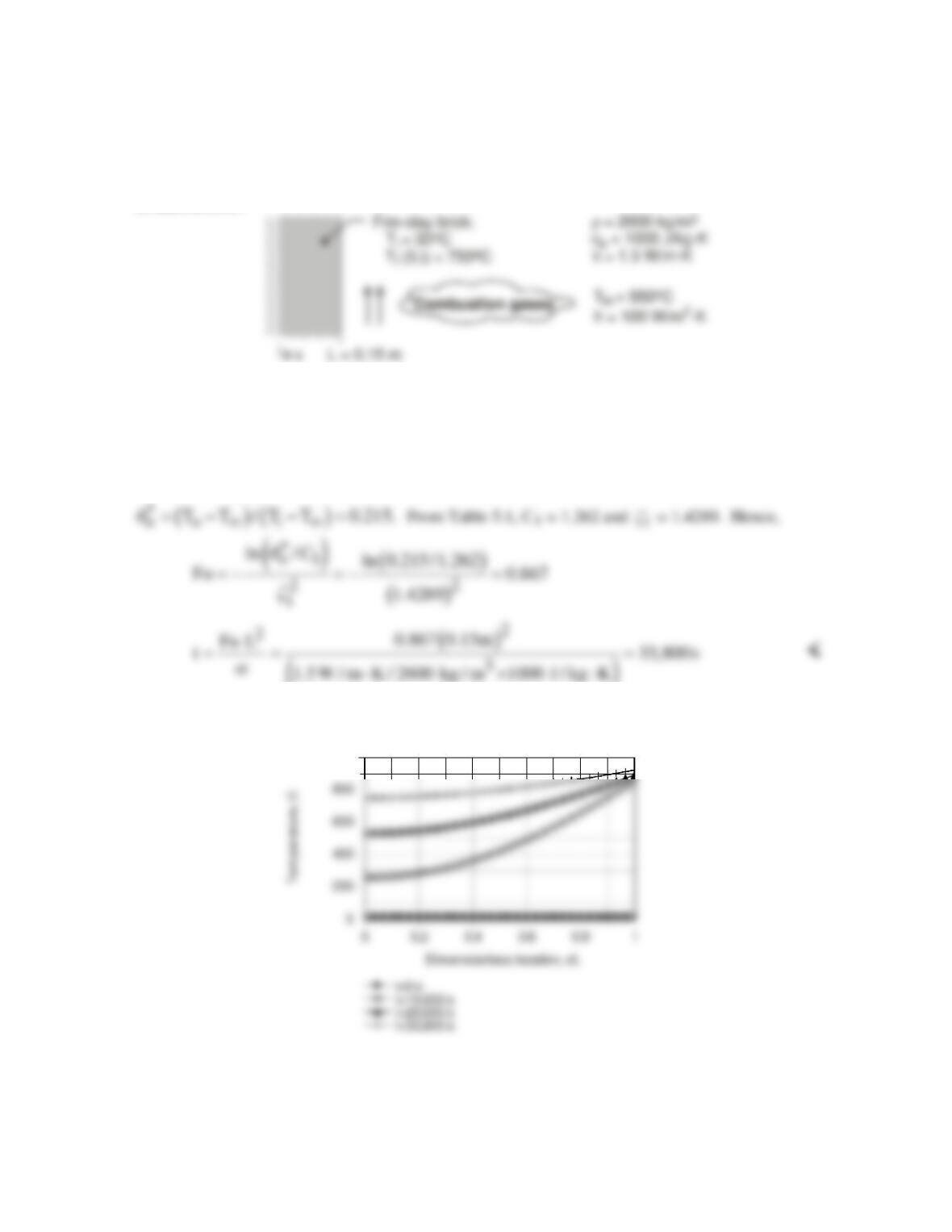
SCHEMATIC:
ASSUMPTIONS: (1) One-dimensional conduction in a plane wall, (2) Constant properties, (3)
Adiabatic outer surface, (4) Fo > 0.2, (5) Negligible radiation from combustion gases.
ANALYSIS: The wall is equivalent to one-half of a wall of thickness 2L with symmetric convection
conditions at its two surfaces. With Bi = hL/k = 100 W/m2⋅K × 0.15m/1.5 W/m⋅K = 10 and Fo > 0.2,
the one-term approximation, Eq. 5.44 may be used to compute the desired time, where
()
The corresponding temperature distribution, as well as distributions at t = 0, 10,000, and 20,000 s are
plotted below
COMMENTS: Because Bi >>1, the temperature at the inner surface of the wall increases much
more rapidly than at locations within the wall, where temperature gradients are large. The
temperature gradients decrease as the wall approaches a steady–state for which there is a uniform
temperature of 950°C.
1000
PROBLEM 5.41
KNOWN: Initial temperature of concrete slabs. Air temperature and convection heat transfer
coefficient.
FIND: Slab thickness required so that Q/Qo = 0.90 for t = 8 h.
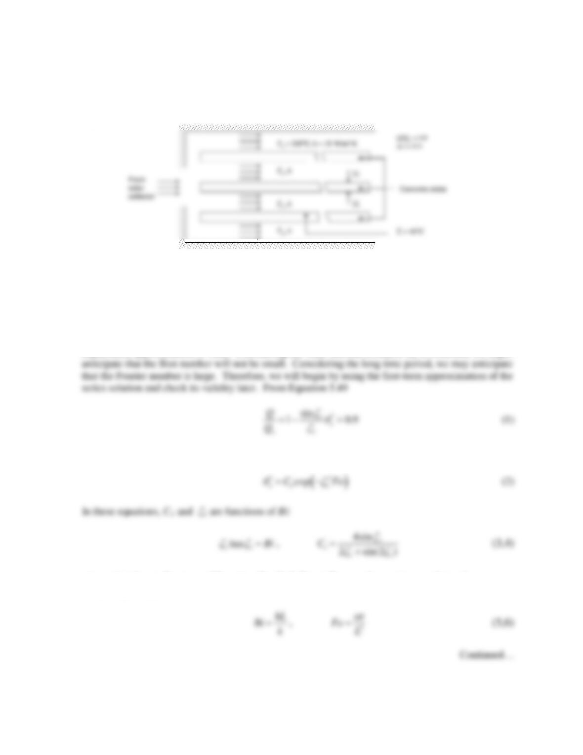
SCHEMATIC:
ASSUMPTIONS: (1) Properties at 300 K are satisfactory at higher temperature, (2) One-dimensional
conduction, (3) Constant convection heat transfer coefficient, (4) Negligible radiation because each
concrete slab is surrounded by others at the same temperature.
PROPERTIES: Table A.3, Concrete (stone mix) (T = 300 K):
ρ
= 2300 kg/m3, c = 880 J/kg⋅K, k =
1.4 W/m⋅K.
ANALYSIS: Without knowing the thickness, we cannot determine in advance whether the lumped
capacitance approximation is valid. Considering the small thermal conductivity of concrete, we might
where from Equation 5.44
where
ζ
1 is the smallest root of Equation (3). Both Bi and Fo are unknown because L is unknown.
They are given by