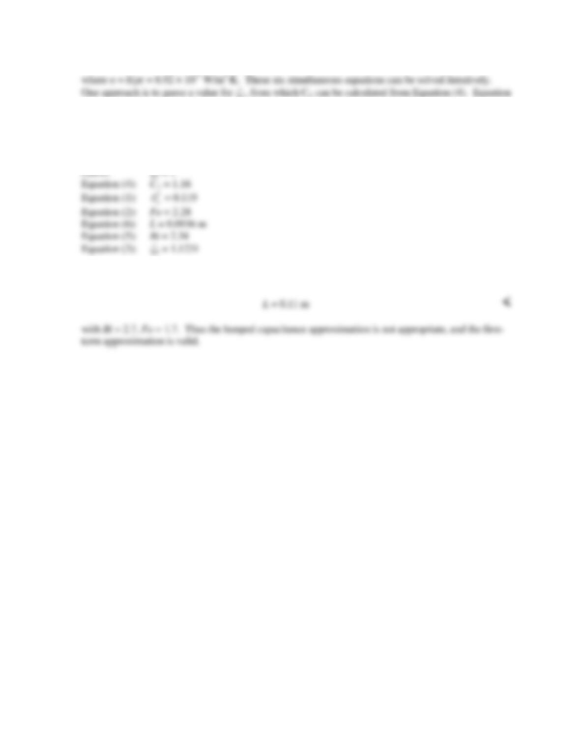
PROBLEM 5.41 (Cont.)
(1) can be used to find the required value of
*
o
θ
. Then Equation (2) can be used to determine Fo and a
new value of L can be determined from Equation (6). Finally, Bi can be calculated from Equation (5)
and a new value of
ζ
1 can be found from Equation (3). Beginning this approach with a guessed value
of
ζ
1 = 1, the iterations proceed as follows:
Repeating with the new value of
ζ
1 and iterating until L converges to two significant digits, we find
COMMENTS: This hand-solution is time-consuming, especially since Equation (3) must itself be
solved iteratively. A much faster approach would be to solve these six equations simultaneously using
IHT or other software.
PROBLEM 5.42
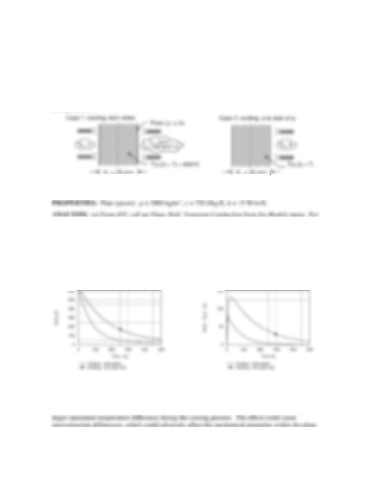
KNOWN: Plate of thickness 2L = 25 mm at a uniform temperature of 600°C is removed from a hot
pressing operation. Case 1, cooled on both sides; case 2, cooled on one side only.
FIND: (a) Calculate and plot on one graph the temperature histories for cases 1 and 2 for a 500-
second cooling period; use the IHT software; Compare times required for the maximum temperature in
the plate to reach 100°C; and (b) For both cases, calculate and plot on one graph, the variation with
time of the maximum temperature difference in the plate; Comment on the relative magnitudes of the
temperature gradients within the plate as a function of time.
SCHEMATIC:
ASSUMPTIONS: (1) One-dimensional conduction in the plate, (2) Constant properties, and (3) For
case 2, with cooling on one side only, the other side is adiabatic.
case 1, the plate thickness is 25 mm; for case 2, the plate thickness is 50 mm. The plate center (x = 0)
temperature histories are shown in the graph below. The times required for the center temperatures to
reach 100°C are
t1 = 164 s t2 = 367 s <
(b) The plot of T(0, t) – T(1, t), which represents the maximum temperature difference in the plate
during the cooling process, is shown below.
Plate center temperature histories
Temperature difference history
COMMENTS: (1) From the plate center–temperature history graph, note that it takes more than twice
as long for the maximum temperature to reach 100°C with cooling on only one side.
(2) From the maximum temperature-difference graph, as expected, cooling from one side creates a
PROBLEM 5.43
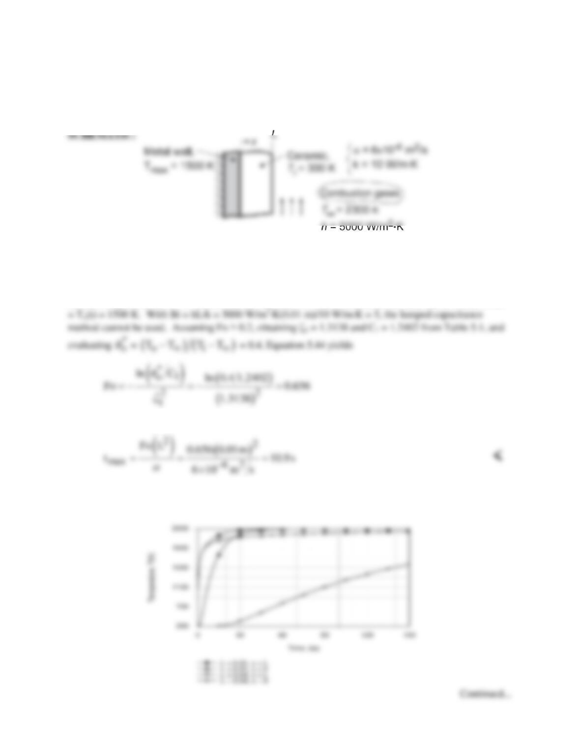
KNOWN: Properties and thickness L of ceramic coating on rocket nozzle wall. Convection conditions.
Initial temperature and maximum allowable wall temperature.
FIND: (a) Maximum allowable engine operating time, tmax, for L = 10 mm, (b) Coating inner and outer
surface temperature histories for L = 10 and 40 mm.
ASSUMPTIONS: (1) One-dimensional conduction in a plane wall, (2) Constant properties, (3)
Negligible thermal capacitance of metal wall and heat loss through back surface, (4) Negligible contact
resistance at wall/ceramic interface, (5) Negligible radiation.
ANALYSIS: (a) Subject to assumptions (3) and (4), the maximum wall temperature corresponds to the
ceramic temperature at x = 0. Hence, for the ceramic, we wish to determine the time tmax at which T(0,t)
confirming the assumption of Fo > 0.2. Hence,
(b) Using the IHT Lumped Capacitance Model for a Plane Wall, the inner and outer surface temperature
histories were computed and are as follows:

PROBLEM 5.43 (Cont.)
The increase in the inner (x = 0) surface temperature lags that of the outer surface, but within t ≈ 45s both
temperatures are within a few degrees of the gas temperature for L = 0.01 m. For L = 0.04 m, the
COMMENTS: The allowable engine operating time increases with increasing thermal capacitance of
the ceramic and hence with increasing L.
PROBLEM 5.44
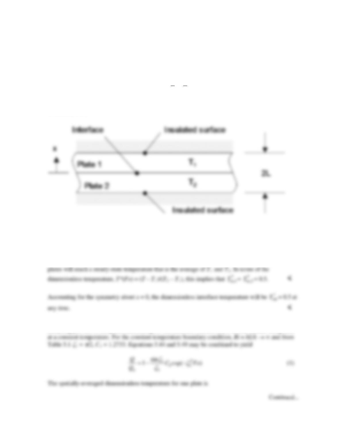
KNOWN: Thickness and initial temperatures of two plates of the same material.
FIND: (a) Steady–state dimensionless temperatures of the two plates,
*
ss,1
Tand
*
ss,2
T
, as well as the
interface temperature,
*
int
T, (b) Expression for the effective dimensionless overall heat transfer
coefficient for the two-plate system,
( )
**
*21
eff ,2 */U qTT≡−
for Fo > 0.2.
SCHEMATIC:
ASSUMPTIONS: (1) One–dimensional conduction, (2) Constant properties, (3) Negligible thermal
contact resistance.
ANALYSIS: (a) Since the two plates are of the same thickness and have the same properties, both
*
*
ss,2
*
int
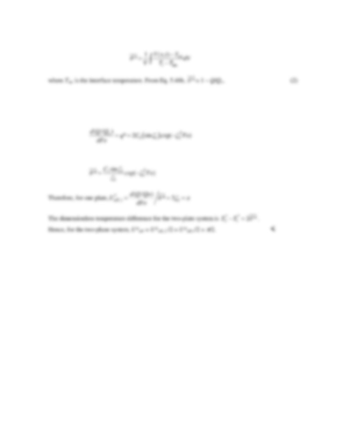
(b) Taking advantage of the geometrical symmetry about x = 0, we may simplify the problem by
analyzing just one of the plates, accounting for one adiabatic surface and a second surface being held
PROBLEM 5.44 (Cont.)
From Eq. (1),
and from Eq. (2)
COMMENTS: (1) For this case, the heat transfer rate between the two plates is proportional to the
difference in the average temperatures of the plates. If Fo < 0.2, it may be shown that U*eff is initially
infinite and decreases with time. This behavior becomes evident if one considers the situation
immediately after the plates make contact when the heat transfer between the plates is very large, but
the average plate temperatures have not been affected significantly by the heat transfer in the vicinity
of the interface. (2) A proportionality between the dimensionless heat transfer rate and the difference
in the average dimensionless plate temperatures also exists at large Fo, even if the plates are not
identical.
PROBLEM 5.45
KNOWN: Initial temperature, thickness and thermal diffusivity of glass plate. Prescribed
surface temperature.
FIND: (a) Time to achieve 75% reduction in midplane temperature, (b) Maximum
temperature gradient at that time.
ASSUMPTIONS: (1) One-dimensional conduction, (2) Constant properties.
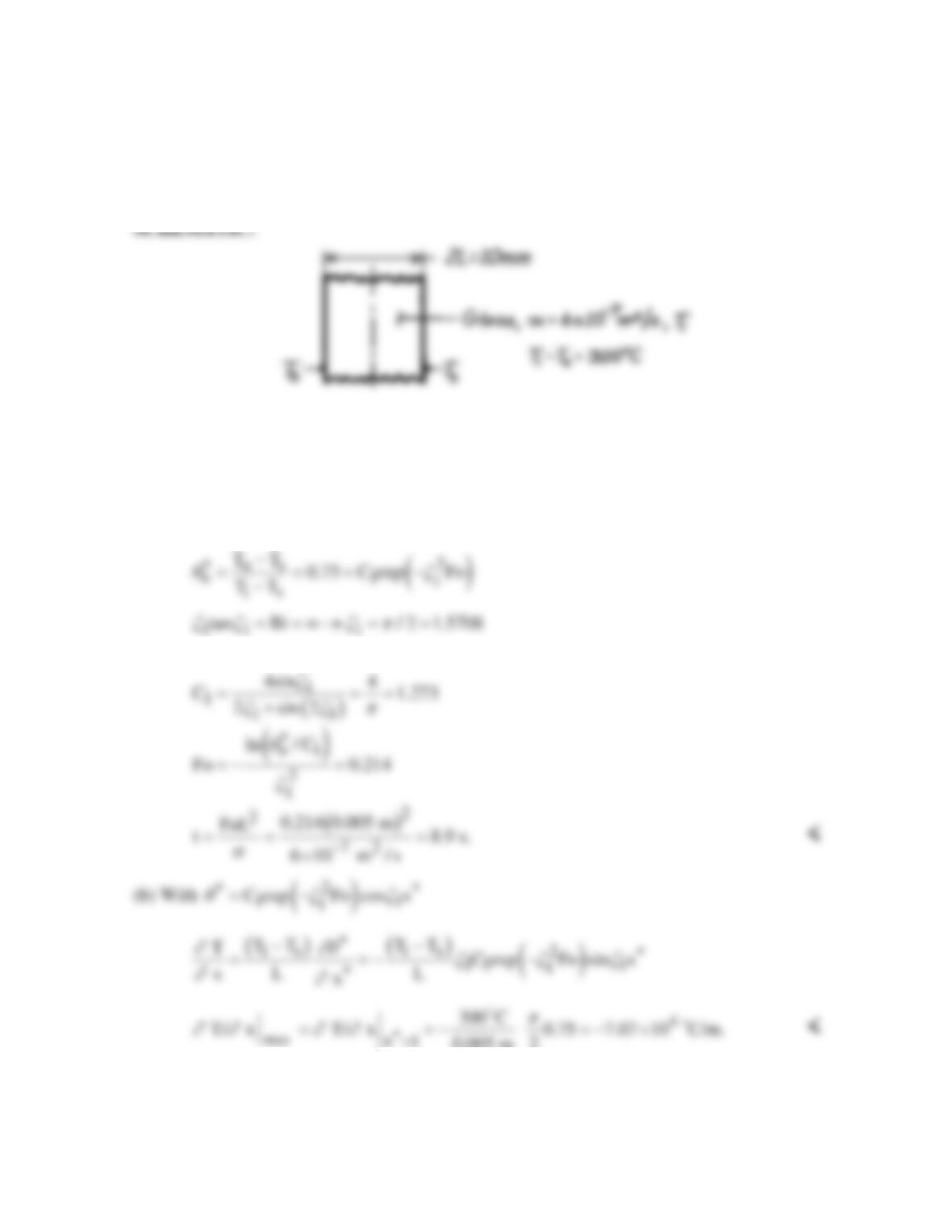
ANALYSIS: Prescribed surface temperature is analogous to h → ∞ and T∞ = Ts. Hence, Bi
= ∞. Assume validity of one-term approximation to series solution for T (x,t).
(a) At the midplane,
Hence
0.005 m 2
COMMENTS: Validity of one-term approximation is confirmed by Fo > 0.2.
PROBLEM 5.46
KNOWN: Thickness and properties of rubber tire. Convection heating conditions. Initial and final
midplane temperature.
FIND: (a) Time to reach final midplane temperature. (b) Effect of accelerated heating.
ASSUMPTIONS: (1) One-dimensional conduction in a plane wall, (2) Constant properties, (3)
Negligible radiation.
ANALYSIS: (a) With Bi = hL/k = 200 W/m2⋅K(0.01 m)/0.14 W/m⋅K = 14.3, the lumped capacitance
method is clearly inappropriate. Assuming Fo > 0.2, Eq. (5.44) may be used with C1 = 1.265 and ζ1 ≈
1.458 rad from Table 5.1 to obtain
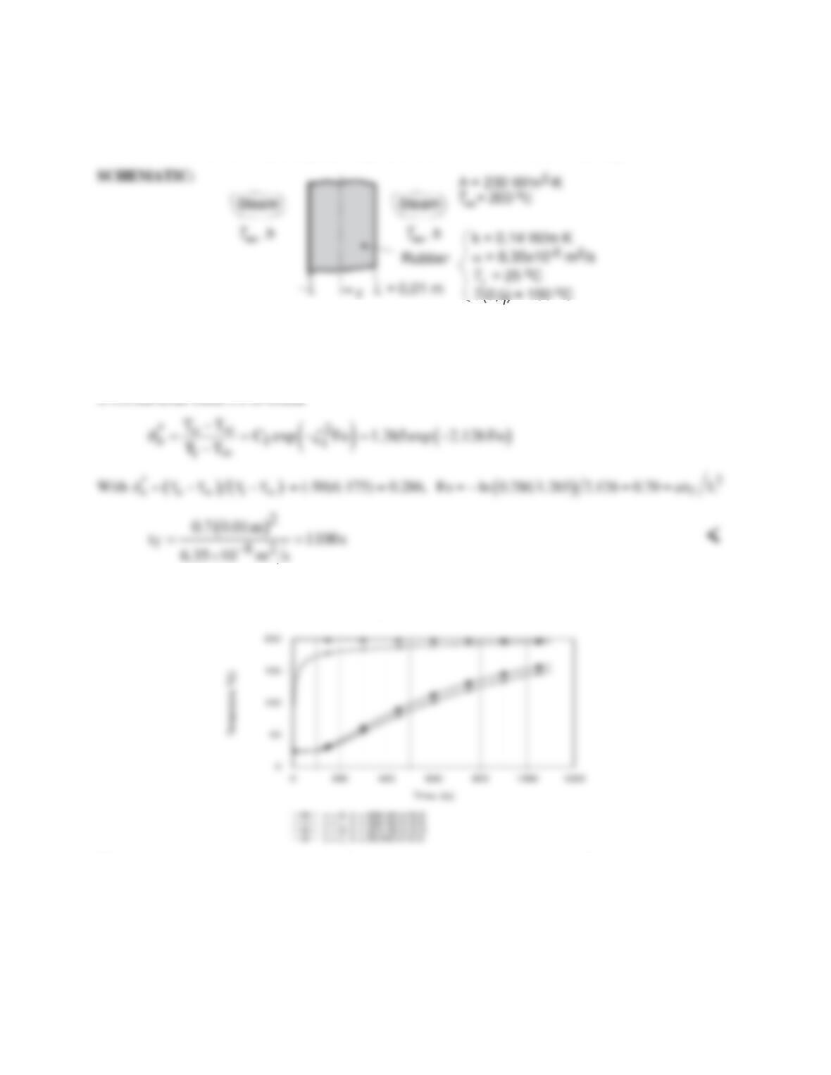
(b) The desired temperature histories were generated using the IHT Transient Conduction Model for a
Plane Wall, with h = 5 × 10⁴ W/m2⋅K used to approximate imposition of a surface temperature of 200°C.
The fact that imposition of a constant surface temperature (h → ∞) does not significantly accelerate the
heating process should not be surprising. For h = 200 W/m2⋅K, the Biot number is already quite large (Bi
= 14.3), and limits to the heating rate are principally due to conduction in the rubber and not to
convection at the surface. Any increase in h only serves to reduce what is already a small component of
the total thermal resistance.
COMMENTS: The heating rate could be accelerated by increasing the steam temperature, but an upper
limit would be associated with avoiding thermal damage to the rubber.
PROBLEM 5.47
KNOWN: Thickness, initial temperature and properties of plastic coating. Safe–to–touch
temperature. Convection coefficient and air temperature.
FIND: Time for surface to reach safe–to-touch temperature. Corresponding temperature at
plastic/wood interface.
ASSUMPTIONS: (1) One-dimensional conduction in coating, (2) Negligible radiation, (3) Constant
properties, (4) Negligible heat of reaction, (5) Negligible heat transfer across plastic/wood interface.
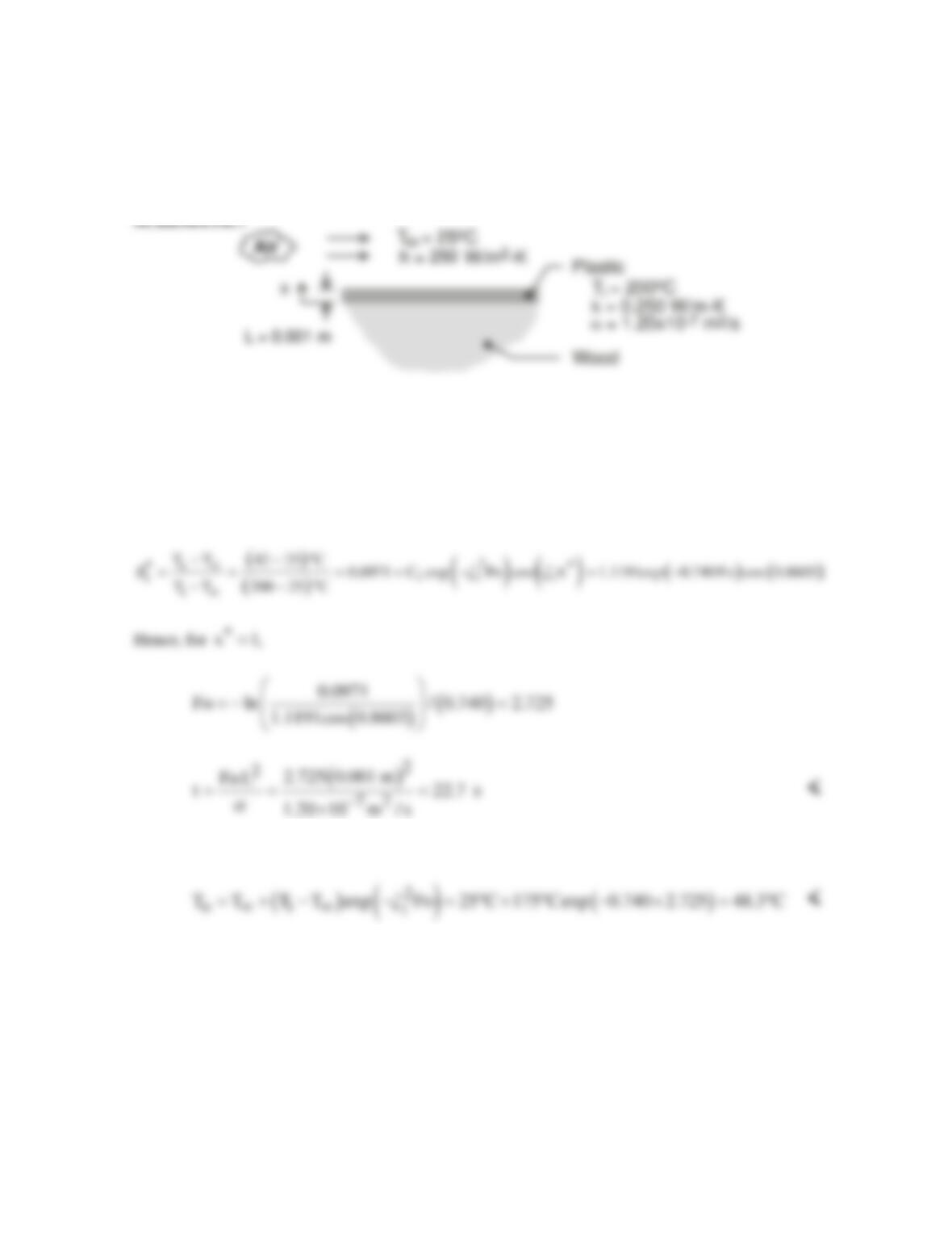
ANALYSIS: With Bi = hL/k = 250 W/m2⋅K × 0.001 m/0.25 W/m⋅K = 1.0 > 0.1, the lumped
capacitance method may not be used. Applying the approximate solution of Eq. 5.43a, with C1 =
1.1191 and
1
ζ
= 0.8603 from Table 5.1,
From Eq. 5.44, the corresponding interface temperature is
COMMENTS: (1) By neglecting conduction into the wood and radiation from the surface, the
cooling time is overpredicted and is therefore a conservative estimate. However, if energy generation
due to solidification of polymer were significant, the cooling time would be longer. (2) The one-term
approximation is valid since Fo > 0.2.
PROBLEM 5.48
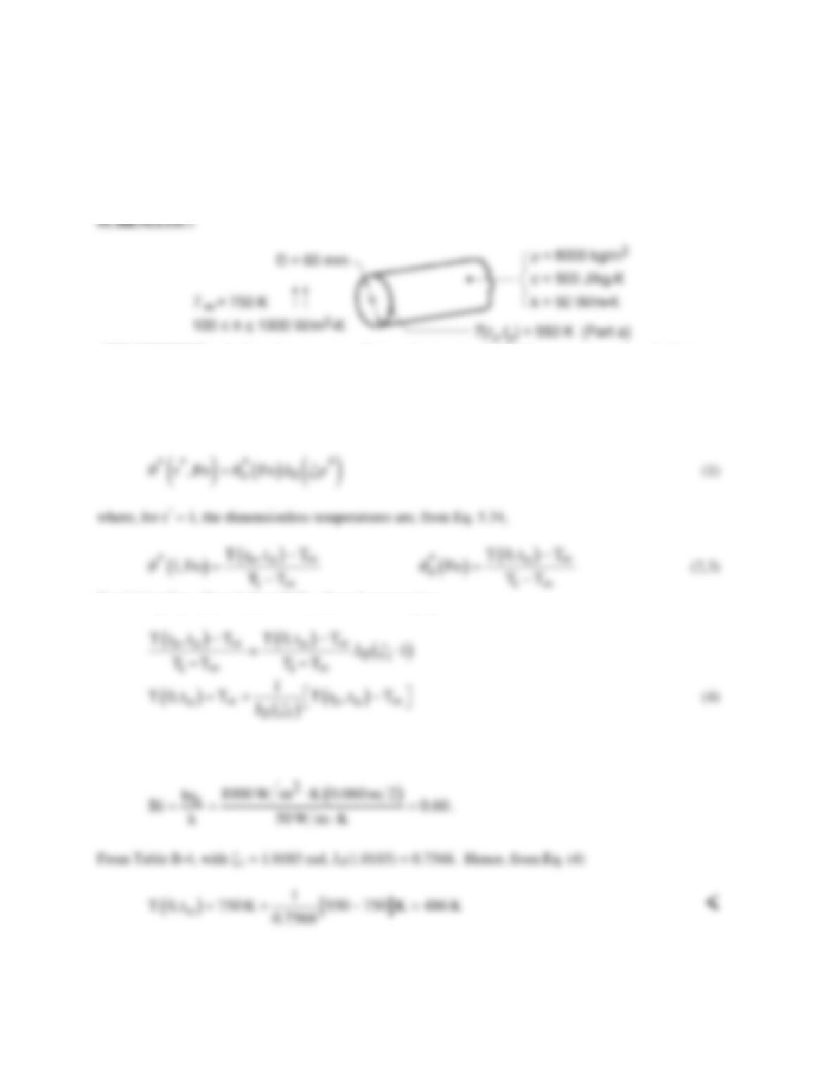
KNOWN: Long rod with prescribed diameter and properties, initially at a uniform temperature, is
heated in a forced convection furnace maintained at 750 K with a convection coefficient of h = 1000
W/m2⋅K.
FIND: (a) The corresponding center temperature of the rod, T(0, to), when the surface temperature T(ro,
to) is measured as 550 K, (b) Effect of h on centerline temperature history.
ASSUMPTIONS: (1) One-dimensional, radial conduction in rod, (2) Constant properties, (3) Rod,
when initially placed in furnace, had a uniform (but unknown) temperature, (4) Fo ≥ 0.2.
ANALYSIS: (a) Since the rod was initially at a uniform temperature and Fo ≥ 0.2, the approximate
solution for the infinite cylinder is appropriate. From Eq. 5.52b,
Combining Eqs. (2) and (3) with Eq. (1) and rearranging,
The eigenvalue, ζ1 = 1.0185 rad, follows from Table 5.1 for the Biot number
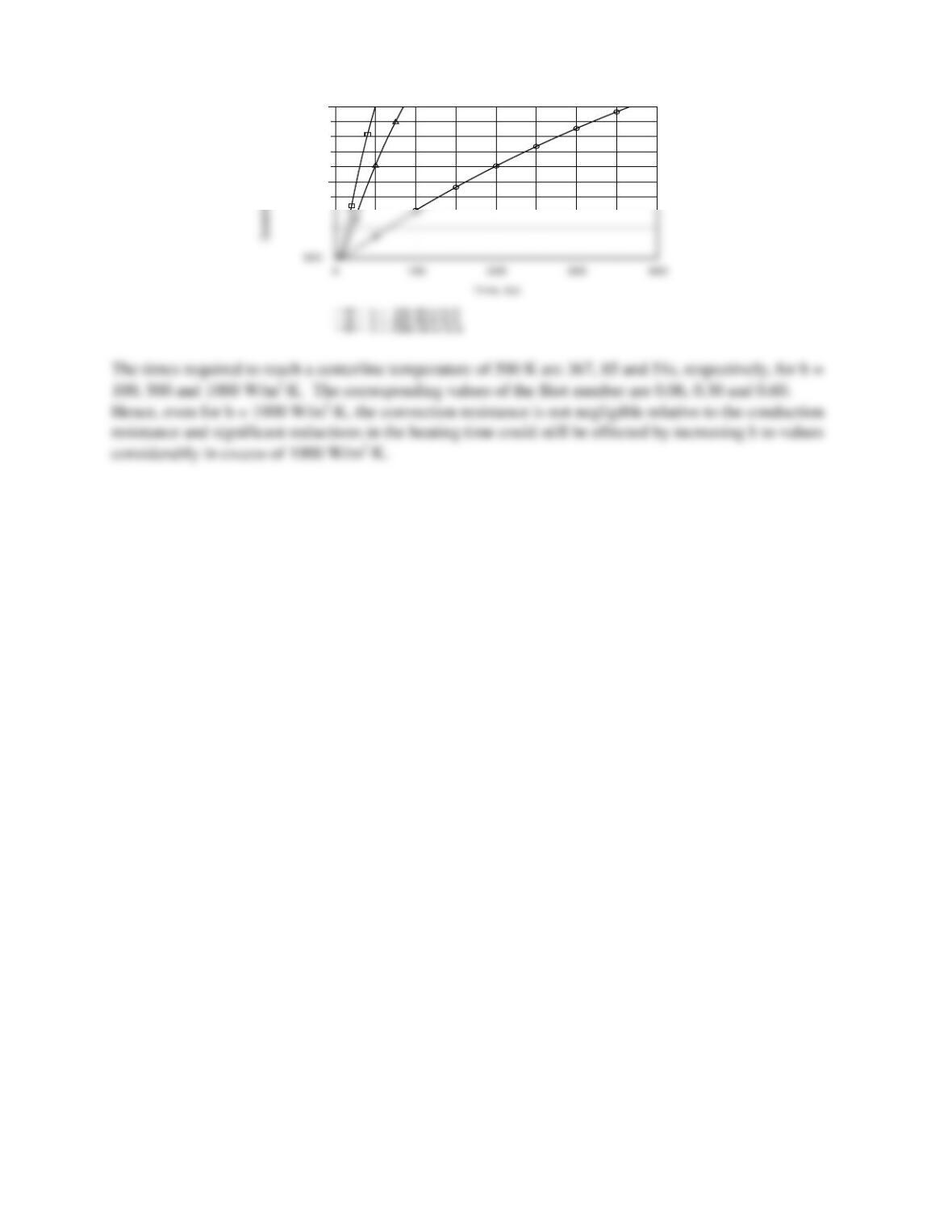
(b) Using the IHT Transient Conduction Model for a Cylinder, the following temperature histories were
generated.
Continued…
PROBLEM 5.48 (Cont.)
400
500
COMMENTS: For Part (a), recognize why it is not necessary to know Ti or the time to. We require
that Fo ≥ 0.2, which for this sphere corresponds to t ≥ 14s. For this situation, the time dependence of the
surface and center are the same.
PROBLEM 5.49
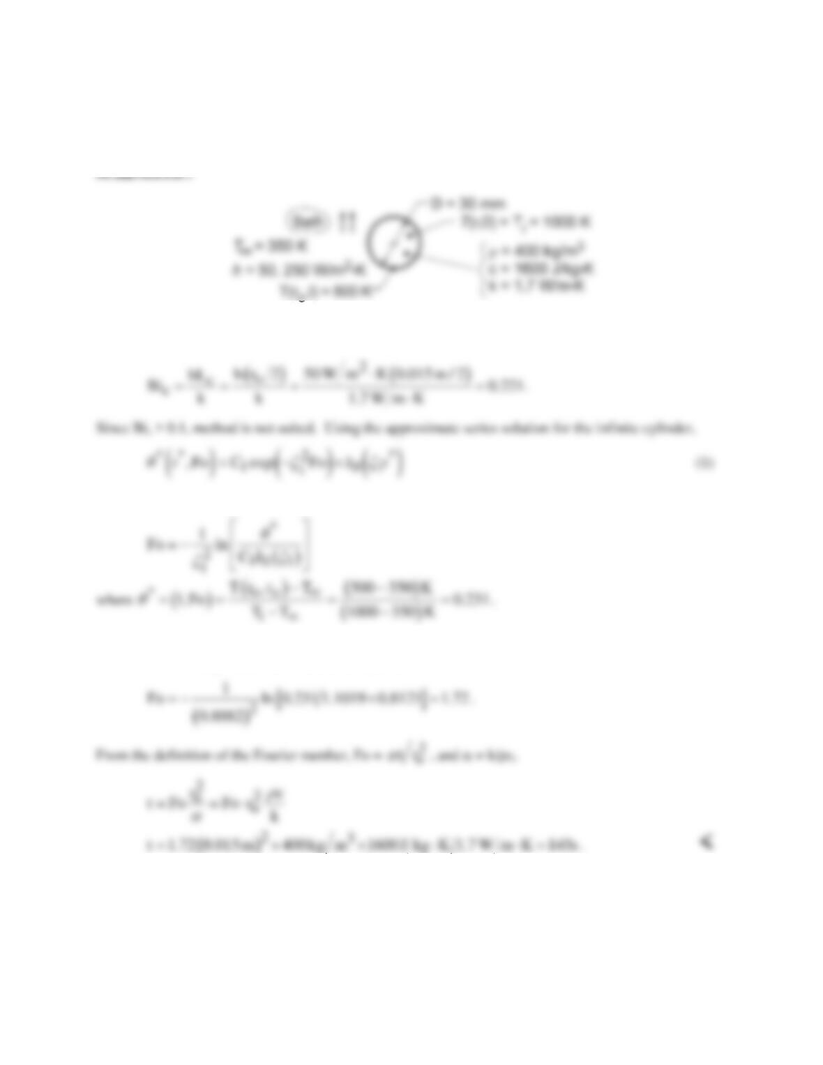
KNOWN: A long cylinder, initially at a uniform temperature, is suddenly quenched in a large oil bath.
FIND: (a) Time required for the surface to reach 500 K, (b) Effect of convection coefficient on surface
temperature history.
ASSUMPTIONS: (1) One-dimensional radial conduction, (2) Constant properties, (3) Fo > 0.2.
ANALYSIS: (a) Check first whether lumped capacitance method is applicable. For h = 50 W/m2⋅K,
Solving for Fo and setting r* = 1, find
From Table 5.1, with Bi = 0.441, find ζ1 = 0.8882 rad and C1 = 1.1019. From Table B.4, find J0(ζ1) =
0.8121. Substituting numerical values into Eq. (2),
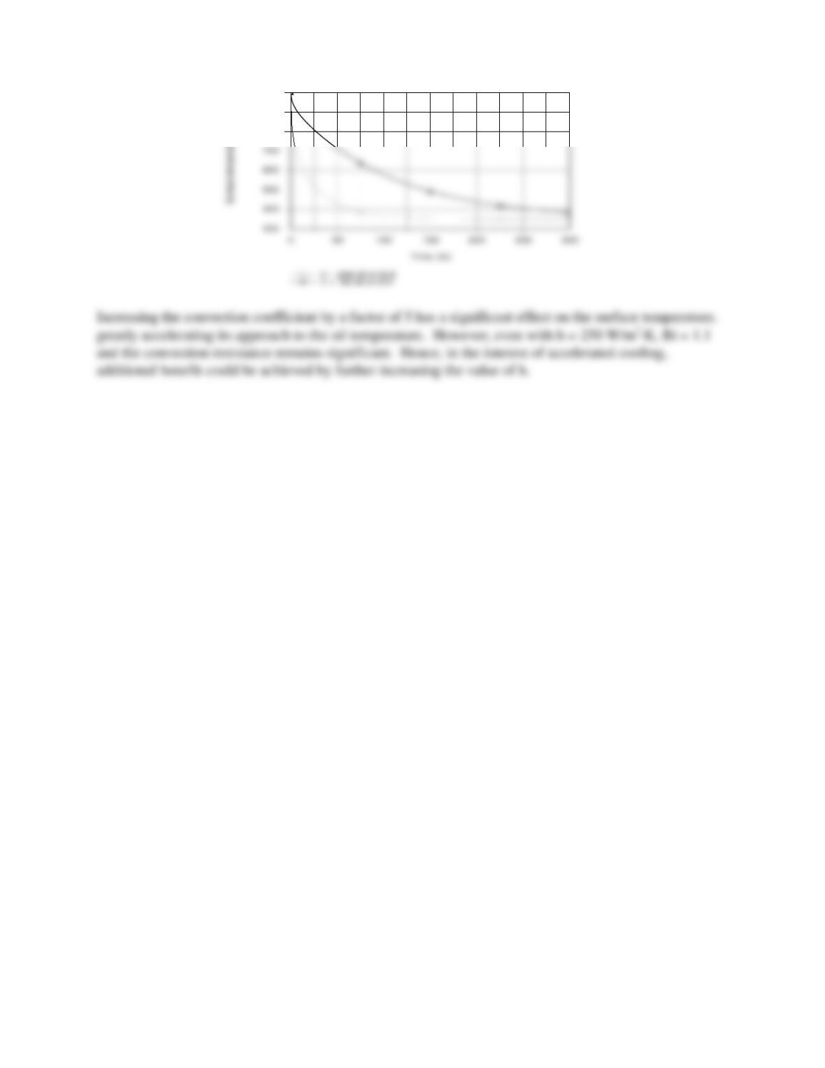
(b) Using the IHT Transient Conduction Model for a Cylinder, the following surface temperature
histories were obtained.
Continued…
PROBLEM 5.49 (Cont.)
800
900
1000
COMMENTS: For Part (a), note that, since Fo = 1.72 > 0.2, the approximate series solution is
appropriate.
PROBLEM 5.50
KNOWN: One-dimensional convective heating of an L/ro = 20 cylinder with Bi = 1 for a
dimensionless time of Fo1.
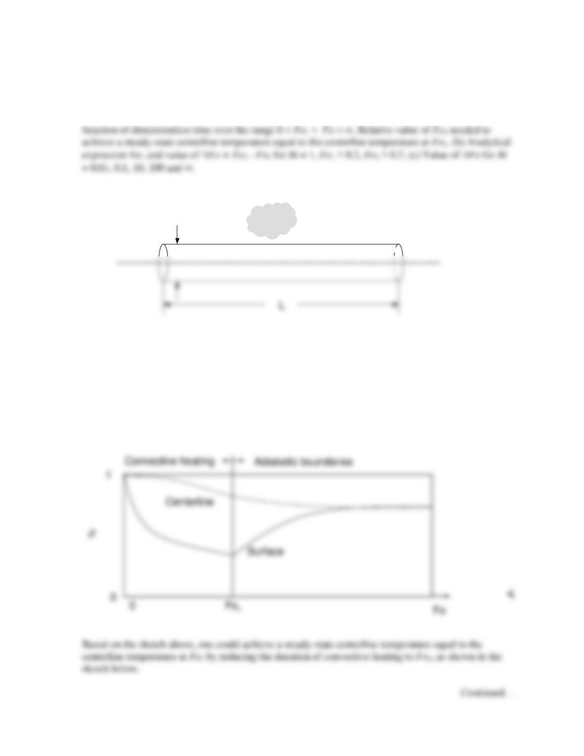
FIND: (a) Sketch of the dimensionless centerline and surface temperatures of the cylinder as a
SCHEMATIC:
ASSUMPTIONS: (1) One-dimensional conduction, (2) Constant properties, (3) Approximate, one-
term solutions are valid.
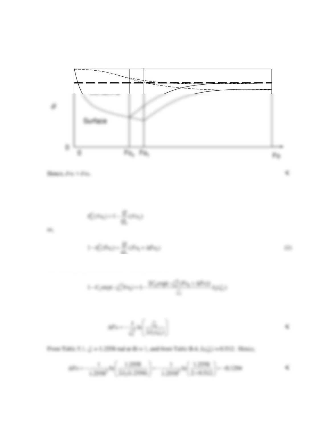
ANALYSIS: (a) A sketch of the dimensionless centerline and surface temperatures is shown below.
Note that, at Fo1, the surface of the cylinder will be warm (smaller
) relative to the centerline since
temperature gradients within the cylinder are significant (Bi = 1). At the curtailment of heating (Fo1),
the surface temperature cools rapidly while warm temperatures continue to propagate toward the
centerline, slowly heating the centerline until a steady-state, isothermal condition is eventually
reached.
2ro
T, h Heating: 0 Fo Fo1
Adiabatic: Fo > Fo1
PROBLEM 5.50 (Cont.)
(b) Using the approximate solutions of Sections 5.6.2 and 5.6.3, and noting that the steady-state
temperature of the cylinder is uniform and related to the energy transferred to the cylinder,
o
Q
Substituting Eqs. 5.52c and 5.54 into Eq. (1) yields
which may be simplified to
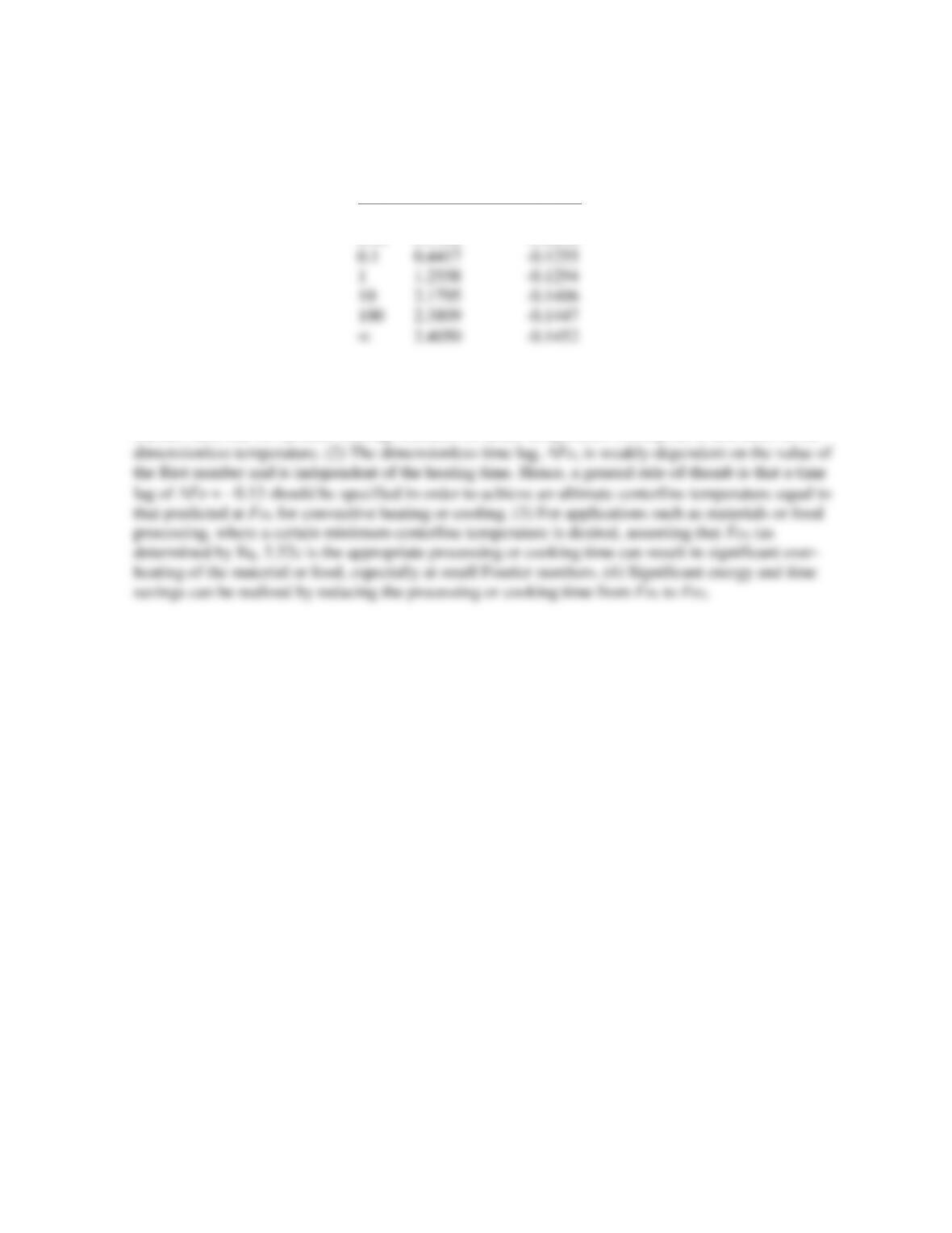
(c) The expression for Fo may be evaluated for a range of Bi, resulting in the following.
Continued…
1
PROBLEM 5.50 (Cont.)
Bi
1 Fo <
0.01 0.1412 -0.1250
COMMENTS: (1) Note that the dimensionless temperature,
*2
11
exp
oC Fo
, is defined in a
manner such that for cylinder heating, increases in actual temperature correspond to decreases in the
PROBLEM 5.51
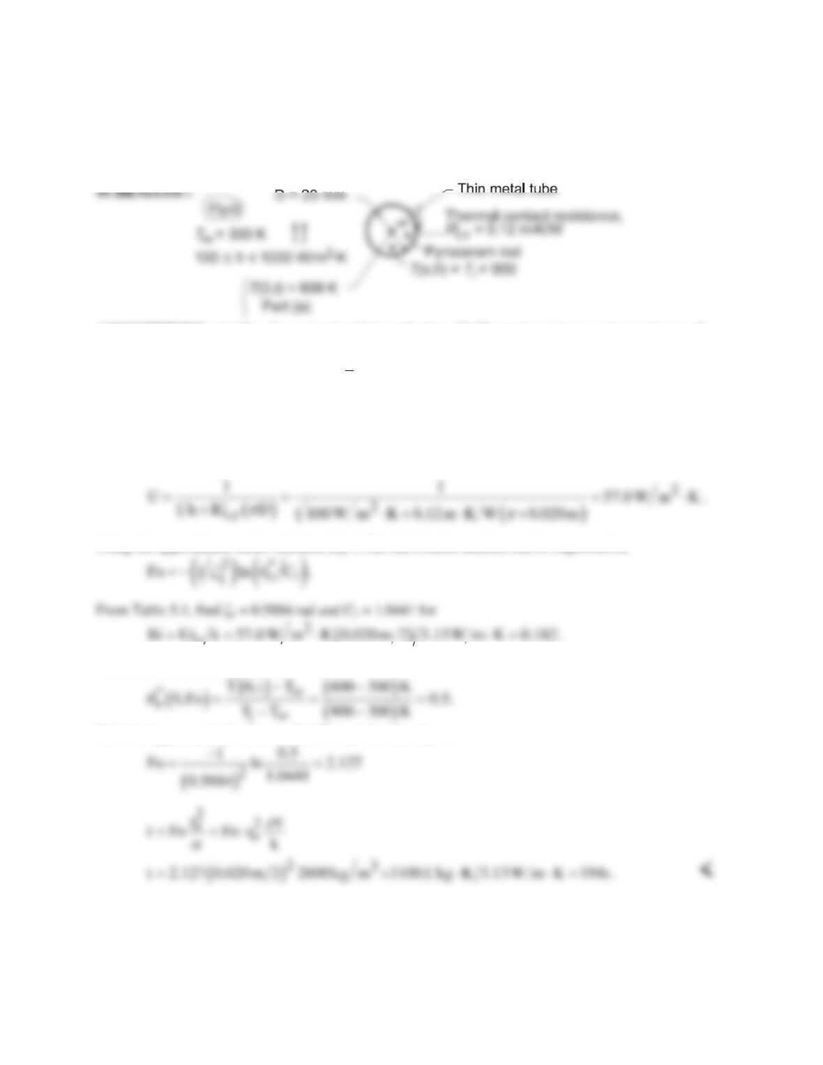
KNOWN: Long pyroceram rod, initially at a uniform temperature of 900 K, and clad with a thin
metallic tube giving rise to a thermal contact resistance, is suddenly cooled by convection.
FIND: (a) Time required for rod centerline to reach 600 K, (b) Effect of convection coefficient on
cooling rate.
ASSUMPTIONS: (1) One-dimensional radial conduction, (2) Thermal resistance and capacitance of
metal tube are negligible, (3) Constant properties, (4) Fo ≥ 0.2.
PROPERTIES: Table A-2, Pyroceram (
T
= (600 + 900)K/2 = 750 K): ρ = 2600 kg/m3, c = 1100
J/kg⋅K, k = 3.13 W/m⋅K.
ANALYSIS: (a) The thermal contact and convection resistances can be combined to give an overall heat
transfer coefficient. Note that
t,c
R′
[m⋅K/W] is expressed per unit length for the outer surface. Hence,
for h = 100 W/m2⋅K,
Using the approximate series solution, Eq. 5.52c, the Fourier number can be expressed as
o
The dimensionless temperature is
Substituting numerical values to find Fo and then the time t,
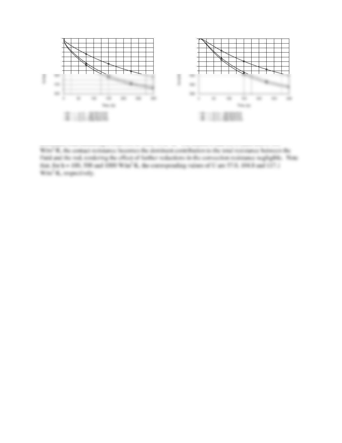
(b) The following temperature histories were generated using the IHT Transient conduction Model for a
Cylinder.
Continued…
PROBLEM 5.51 (Cont.)
600
700
800
900
600
700
800
900
While enhanced cooling is achieved by increasing h from 100 to 500 W/m2⋅K, there is little benefit
associated with increasing h from 500 to 1000 W/m2⋅K. The reason is that for h much above 500
COMMENTS: For Part (a), note that, since Fo = 2.127 > 0.2, Assumption (4) is satisfied.
PROBLEM 5.52
KNOWN: Sapphire rod, initially at a uniform temperature of 800 K is suddenly cooled by a
convection process; after 35 s, the rod is wrapped in insulation.
FIND: Temperature rod reaches after a long time following the insulation wrap.
SCHEMATIC:
ASSUMPTIONS: (1) One-dimensional radial conduction, (2) Constant properties, (3) No heat losses
from the rod when insulation is applied.
PROPERTIES: Table A-2, Aluminum oxide, sapphire (550K): ρ = 3970 kg/m3, c = 1068 J/kg⋅K, k
= 22.3 W/m⋅K, α = 5.259×10⁻⁶ m2/s.
ANALYSIS: First calculate the Biot number with Lc = ro/2,
Eventually (t → ∞), the temperature of the rod will be uniform at
( )
T.∞
We begin by determining the energy transferred from the rod at t = 35 s. We have
o
Since Fo > 0.2, we can use the one-term approximation. From Table 5.1, ζ1 = 1.4036 rad, C1 =
1.2636. Then from Equation 5.49c,
PROBLEM 5.52 (Cont.)
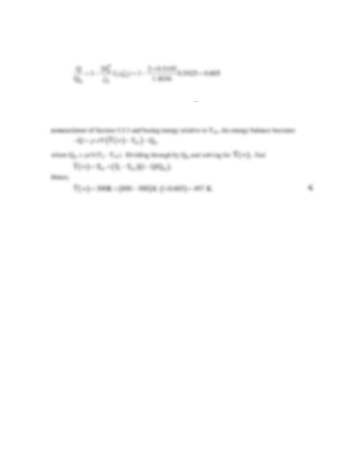
where J1(ζ1) was found from App. B.4. Since the rod is well insulated after t = 35 s, the energy
transferred from the rod remains unchanged. To find
( )
T,∞
write the conservation of energy
requirement for the rod on a time interval basis,
in out final initial
E E EE E .− =∆≡ −
Using the