Section 7.3: The Eigenvalue Method for Linear Systems 415
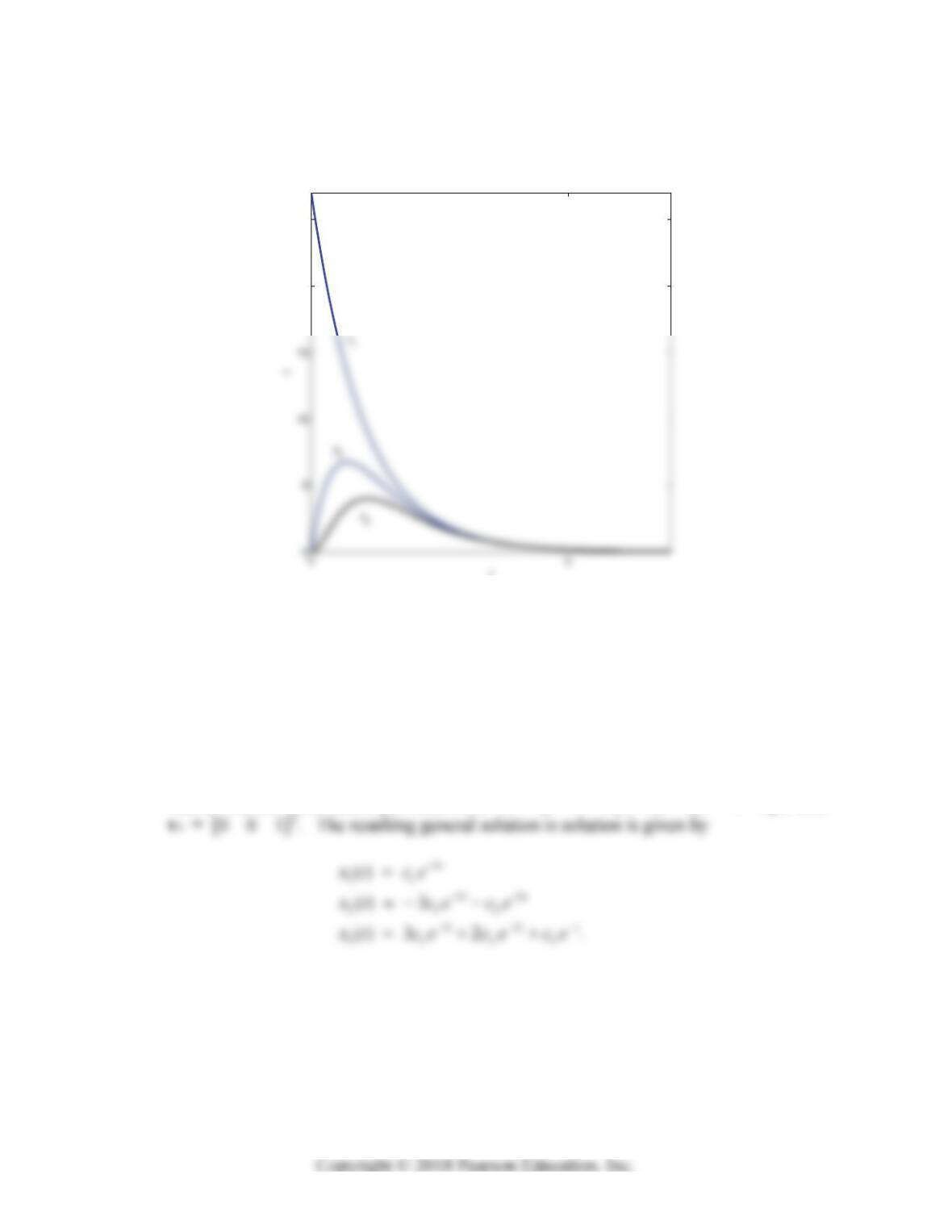
with positive solution ln 3.
m
t Thus the maximum amount of salt ever in tank 3 is
3(ln 3) 4x pounds. The figure below shows the graphs of 12 3
( ), ( ), and ( ).
x
txt xt
20
25
t
32. The coefficient matrix
30 0
320
02 1
A
has as eigenvalues its diagonal elements
1 = –3,
2 = –2, and
3 = –1. We find
readily that the associated eigenvectors are v1 = [1 –3 3]T, v2 = [0 –1 2]T, and
x
The initial conditions 122
(0) 45, (0) (0) 0xxx give 12 3
45, 135, 135,cc c
so we get
3
1
32
2
32
3
() 45
( ) 135 135
( ) 135 270 135 .
t
tt
ttt
xt e
xt e e
x
teee
416 Chapter 7: Linear Systems of Differential Equations
The equation 3() 0xt
simplifies to the equation
2
34131 10
tt t t
ee e e
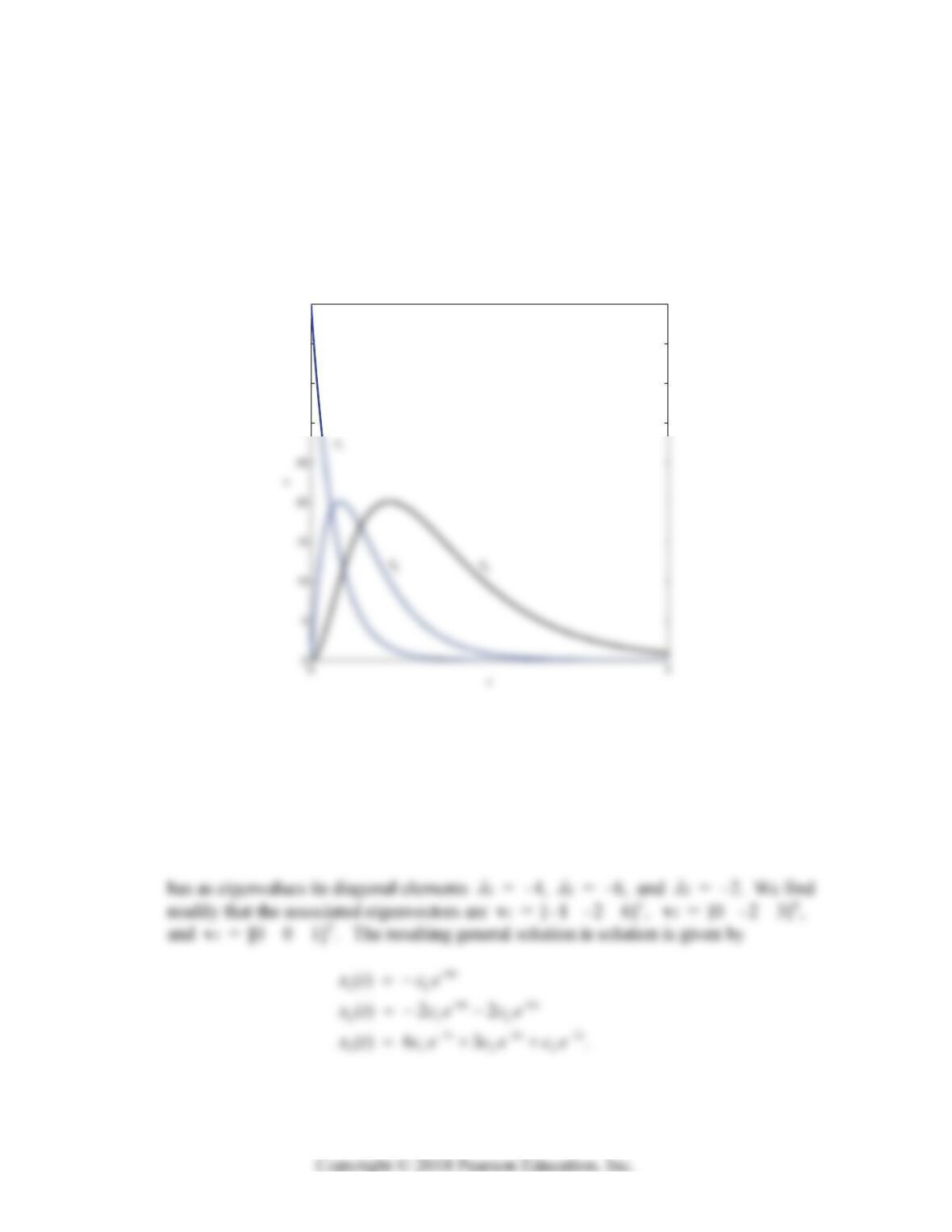
with positive solution ln 3.
m
t Thus the maximum amount of salt ever in tank 3 is
320
(ln 3)x pounds. The figure below shows the graphs of 12 3
( ), ( ), and ( ).
x
txt xt
30
35
40
45
33. The coefficient matrix
40 0
460
06 2
A
x
Section 7.3: The Eigenvalue Method for Linear Systems 417
The initial conditions 122
(0) 45, (0) (0) 0xxx give 123
45, 45, 135,ccc so
we get
The equation 3() 0xt
simplifies to the equation
25
30
35
40
45
t
x
1
34. The coefficient matrix
30 0
350
05 1
A
418 Chapter 7: Linear Systems of Differential Equations
3
11
35
212
35
3123
() 4
() 6 4
() 15 5 .
t
tt
ttt
xt ce
xt ce ce
x
tcecece
x
The equation 3() 0xt
simplifies to the equation
42 2 2
56151 10
tt t t
ee e e
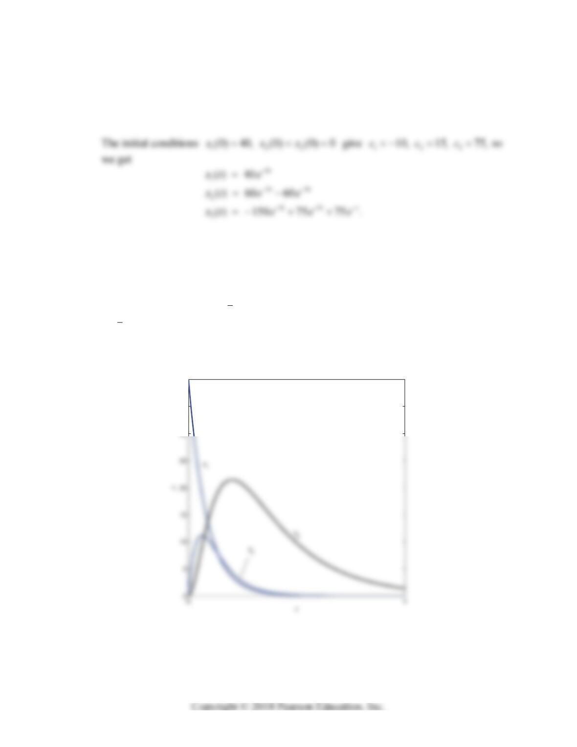
with positive solution 1
2ln 5.
m
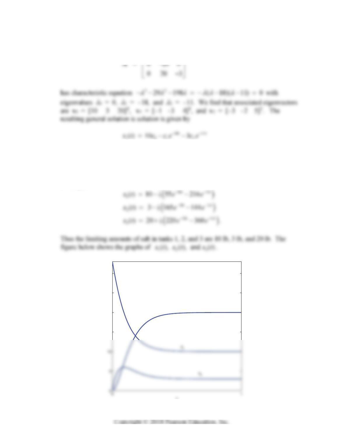
t Thus the maximum amount of salt ever in tank 3 is
1
2
3( ln 5) 21.4663x pounds. The figure below shows the graphs of 12
(), (),
x
txt
3
and ( )
x
t.
30
35
40
Section 7.3: The Eigenvalue Method for Linear Systems 419
35. The coefficient matrix
60 3
18 11
201 2
18 11
3012
() 3 3 2
() 20 4 5 .
tt
tt
xt c ce ce
xt c ce ce
The initial conditions 122
(0) 33, (0) (0) 0xxx give 12 3
1, 55 / 7, 72 / 7,cc c
so we get
15
20
25
30
t
x
x
3
420 Chapter 7: Linear Systems of Differential Equations
36. The coefficient matrix
11
22
11
25
11
52
0
0
0
A
associated with the eigenvalue
0 = 0 yields the associated eigenvector
v0 = [1 5/2 1]T and consequently the constant solution 00
() .txv Then the
eigenvector equation
(63) /10
11
3/5
()
cos(3 /10) 3sin(3 /10) 3cos(3 /10) sin(3 /10)
1cos(3 /10) 3sin(3 /10) 3cos(3 /10) sin(3 /10) .
22cos(3 /10) 2 sin(3 /10)
it
t
te
ttitt
ettitt
tit
xv
The scalar components of resulting general solution 00 1 1 2 1
Re( ) Im( )cc c xx x x are
given by
Section 7.3: The Eigenvalue Method for Linear Systems 421
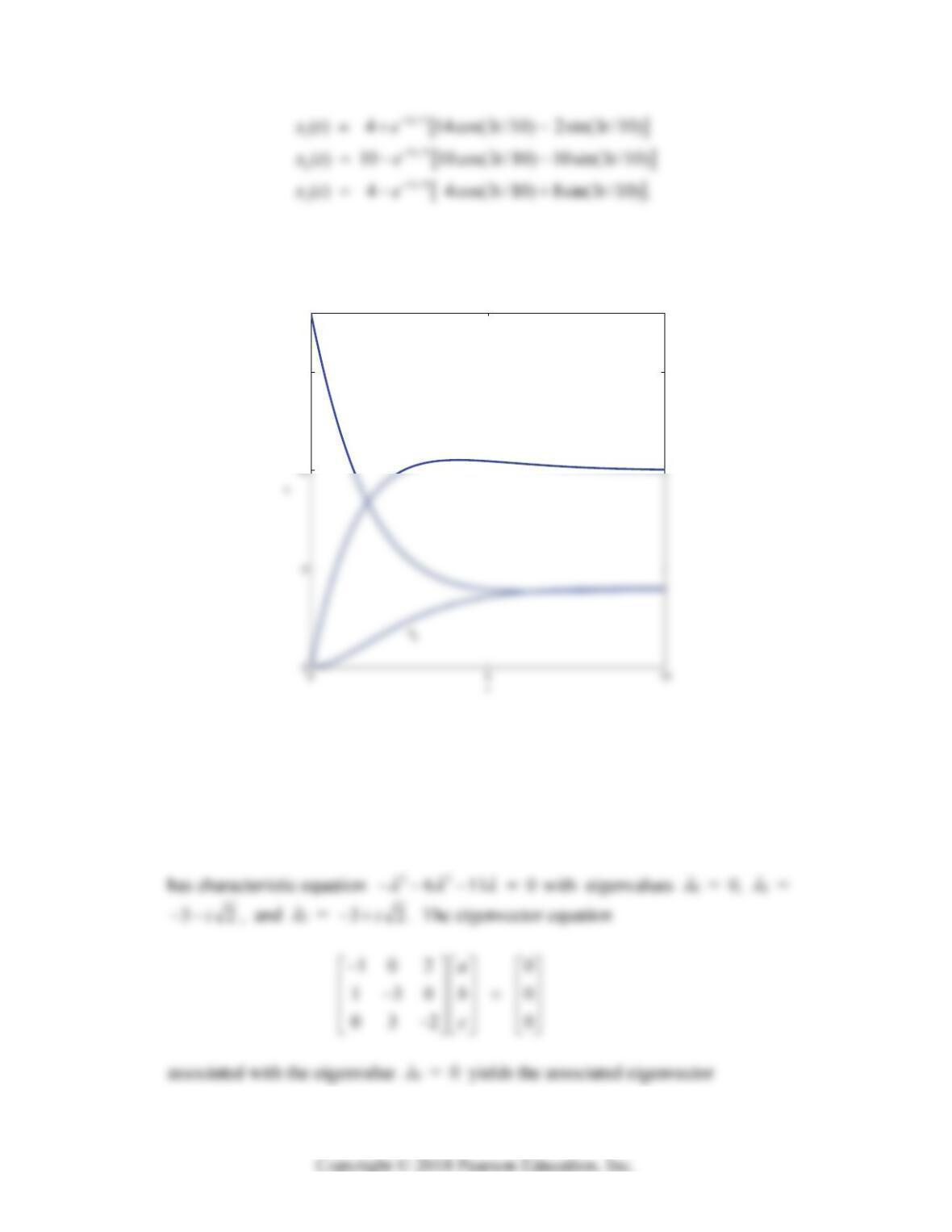
Thus the limiting amounts of salt in tanks 1, 2, and 3 are 4 lb, 10 lb, and 4 lb. The figure
below shows the graphs of 12
(), (),
x
txt 3
and ( )
x
t.
15
x
1
x
2
37. The coefficient matrix
10 2
130
03 2
A
422 Chapter 7: Linear Systems of Differential Equations
v0 = [6 2 3]T and consequently the constant solution 00
() .txv Then the
eigenvector equation
associated with
1 = 32i yields the complex-valued eigenvector
T
1(2 2)/3 (1 2)/3 1ii
v. The corresponding complex-valued solution
is
The scalar components of resulting general solution 00 1 1 2 1
Re( ) Im( )cc c xx x x are
given by
When we impose the initial conditions 122
(0) 55, (0) (0) 0xxx we find that
01 2
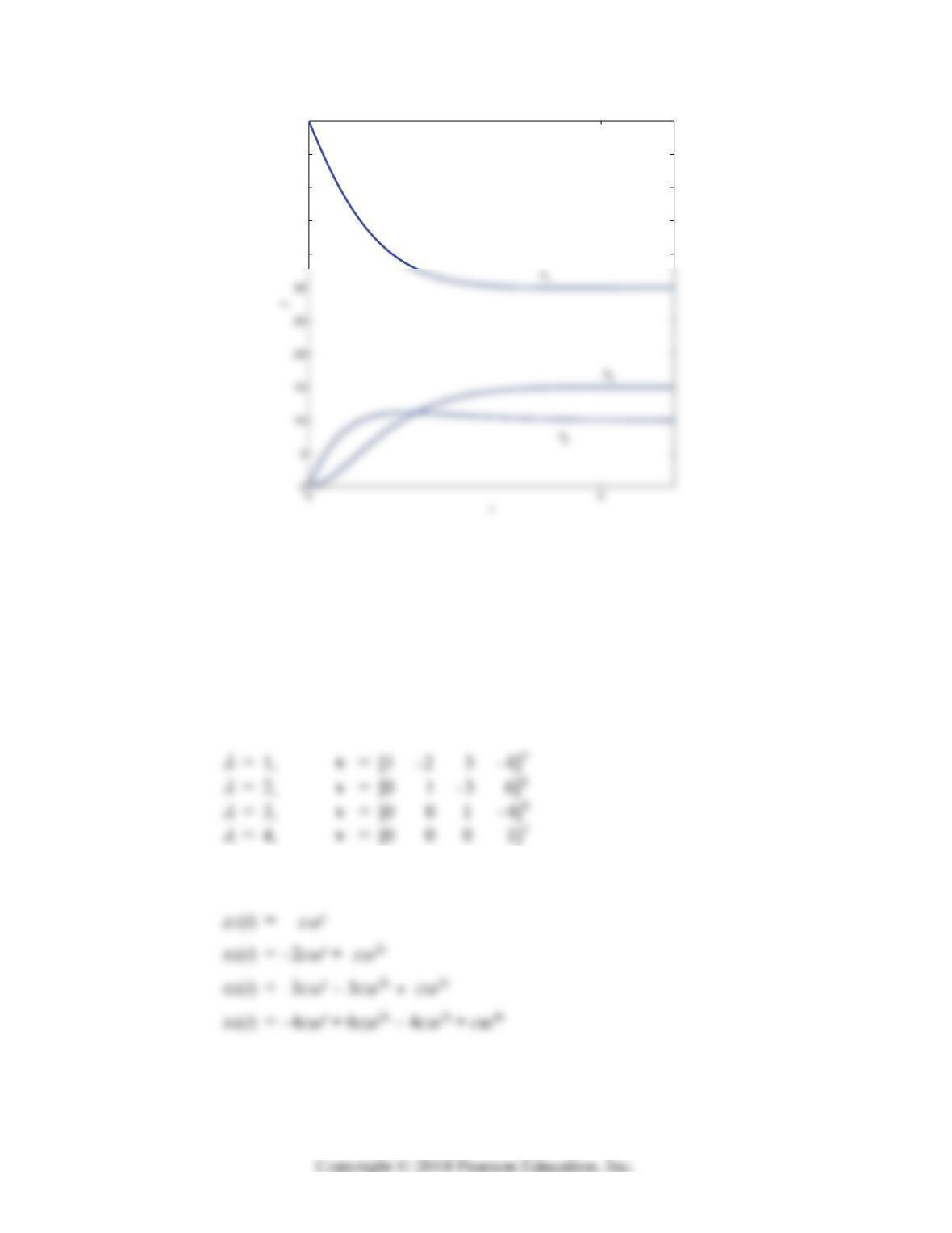
5, 15, and 45/ 2.cc c This finally gives the particular solution
Section 7.3: The Eigenvalue Method for Linear Systems 423
35
40
45
50
55
In Problems 38–41 the Maple command with(linalg):eigenvects(A), the Mathematica
command Eigensystem[A], or the MATLAB command [V,D] = eig(A) can be used to
find the eigenvalues and associated eigenvectors of the given coefficient matrix A.
38. Characteristic equation: (
– 1)(
– 2)(
– 3)(
– 4) = 0
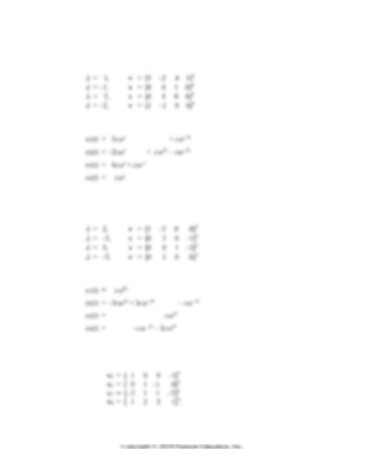
Eigenvalues and associated eigenvectors:
Scalar solution equations:
424 Chapter 7: Linear Systems of Differential Equations
39. Characteristic equation: (
2 – 1)(
2 – 4) = 0
Eigenvalues and associated eigenvectors:
Scalar solution equations:
40. Characteristic equation: (
2 – 4)(
2 – 25) = 0
Eigenvalues and associated eigenvectors:
Scalar solution equations:
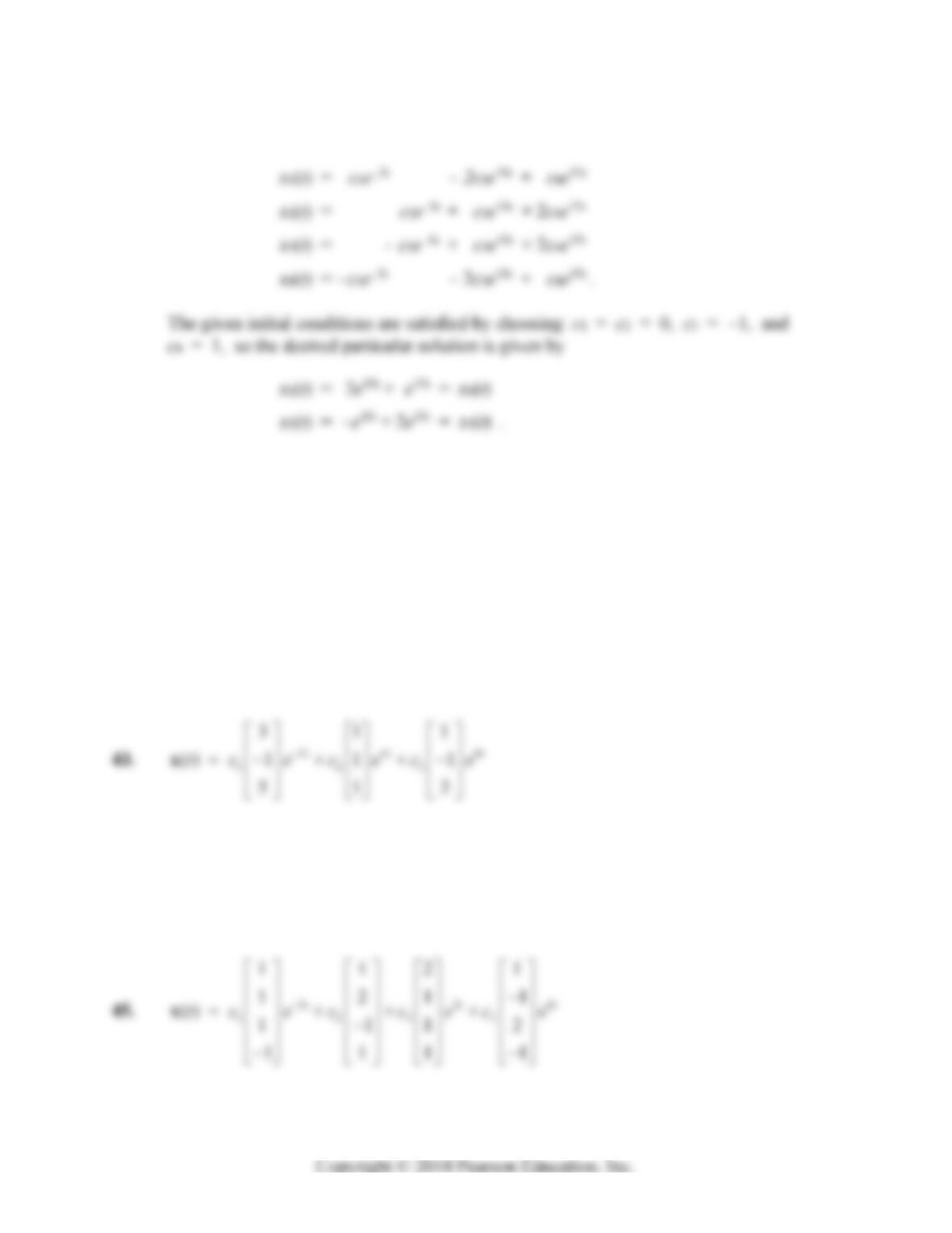
41. The eigenvectors associated with the respective eigenvalues
1 = –3,
2 = –6,
3 = 10, and
4 = 15 are
Section 7.3: The Eigenvalue Method for Linear Systems 425
Hence the general solution has scalar component functions
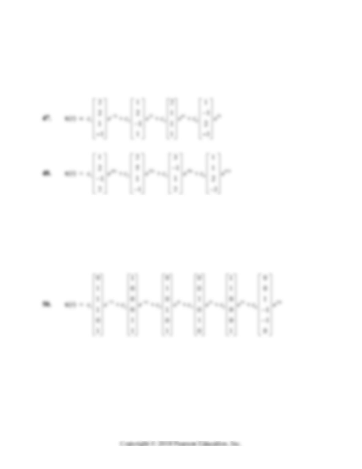
In Problems 42–50 we give a general solution in the form 12
11 2 2
() tt
tce ce
xv v that
exhibits explicitly the eigenvalues 12
,,
and corresponding eigenvectors 12
,,vv of the
given coefficient matrix A.
42. 25
12 3
31 2
() 1 1 3
21 1
tt
tc cec e
x
44. 36 12
123
375
() 2 1 3
253
tt t
tc ec ec e
x
426 Chapter 7: Linear Systems of Differential Equations
46. 4248
1234
3113
2212
() 12 13
1113
tttt
tc ec ec ec e
x
49. 3369
12345
10102
03710
() 30105
11112
11111
tttt
tcec cecece
x
Section 7.4: A Gallery of Solution Curves of Linear Systems 427
SECTION 7.4
A GALLERY OF SOLUTION CURVES OF LINEAR SYSTEMS
This section emphasizes the connection between the algebraic properties of the matrix A—
specifically, its eigenvalues and eigenvectors—and the characteristic pattern of the phase
diagram of the system xAx
.
In Problems 1-16 the eigenvalues, eigenvectors and phase portraits appear in the solutions to
Section 7.3. Thus here we simply categorize each phase portrait according to the gallery in Fig.
7.4.16.
1. Saddle point (real eigenvalues of opposite sign)
5. Saddle point (real eigenvalues of opposite sign)
6. Improper nodal source (distinct positive real eigenvalues)
7. Saddle point (real eigenvalues of opposite sign)
11. Spiral source (complex conjugate eigenvalues with positive real part)
12. Spiral source (complex conjugate eigenvalues with positive real part)
13. Spiral source (complex conjugate eigenvalues with positive real part)
428 Chapter 7: Linear Systems of Differential Equations
In Problems 17-28 we “pigeonhole” each phase portrait according to the gallery in Fig. 7.4.16
and give the nature of the eigenvalues of the matrix A. Where appropriate we further give
approximate values of the corresponding eigenvectors.
17. Center; pure imaginary eigenvalues
20. Spiral source; complex conjugate eigenvalues with positive real part
21. Proper nodal source; repeated positive real eigenvalue with linearly independent
eigenvectors
22. Parallel lines; one zero and one negative real eigenvalue
25. Saddle point; real eigenvalues of opposite sign;
T
111v corresponds to the positive
26. Center; pure imaginary eigenvalues
27. Improper nodal source; distinct positive real eigenvalues;
T
123v ,
T
221v
28. Spiral sink; complex conjugate eigenvalues with negative real part
Section 7.4: A Gallery of Solution Curves of Linear Systems 429
30. The chain rule for vector-valued functions, together with the definition of
tx
as
tx,
gives
.
31. If
is an eigenvalue of A with associated eigenvector v, then
AIv0
. Taking
the negative of both sides of this equation then gives
AIv00. However,
32. If we suppose that the system xAx has a nonzero constant solution x, then
0
d
dt
xx for all t, which means that 0Ax. Hence x is a nonzero constant vector
33. a) Let 1
v and 2
v denote the two linearly independent eigenvectors of A associated with
the eigenvalue
, so that 11
Av v and 22
Av v . If v is any two-dimensional vector,
then the fact that 1
v and 2
v are linearly independent implies that v can be written as a
linear combination of 1
v and 2
v, so that 11 2 2
ccvv v for some scalars 1
c and 2
c. But
430 Chapter 7: Linear Systems of Differential Equations
34. Substituting the expressions for
1
x
t and
2
x
t into the expressions for u and v gives
35. Write the given equation as
12 1 12 2
,,0Mxx dx Nxx dx, where
12 2 1
,68
M
xx x x
and
12 1 2
,617Nxx x x . The equation is exact because
21
6
M
N
x
x
. Its general solution is therefore given by
12
,Fxx k, where
12
,Fxx
(as discussed in Section 1.6) satisfies the conditions
x
F
M
FN
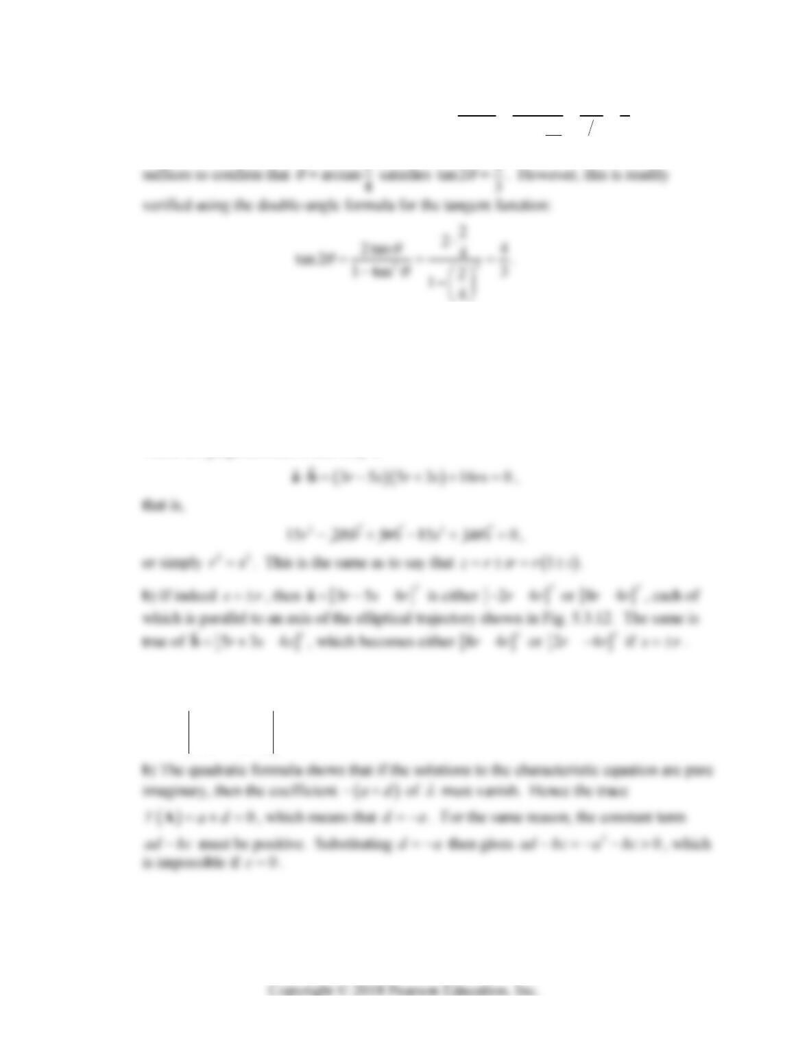
36. Taking 4A , 6B, and 17
2
C gives 22
17
4 6 4 4 100 0
2
BAC. Thus
the nontrivial solution curves are indeed elliptical.
Section 7.4: A Gallery of Solution Curves of Linear Systems 431
37. With the same values of A, B, and C we find that 664
17 92 3
42
B
AC
. Thus it
38. a) Let zrsi , so that
35
35 35 53
4
444
Trsi i
irsirs
zrsi
rsi rsi
vv
has real and imaginary parts
354
T
rsra
and
534
T
rssb
, respectively.
These are perpendicular if and only if
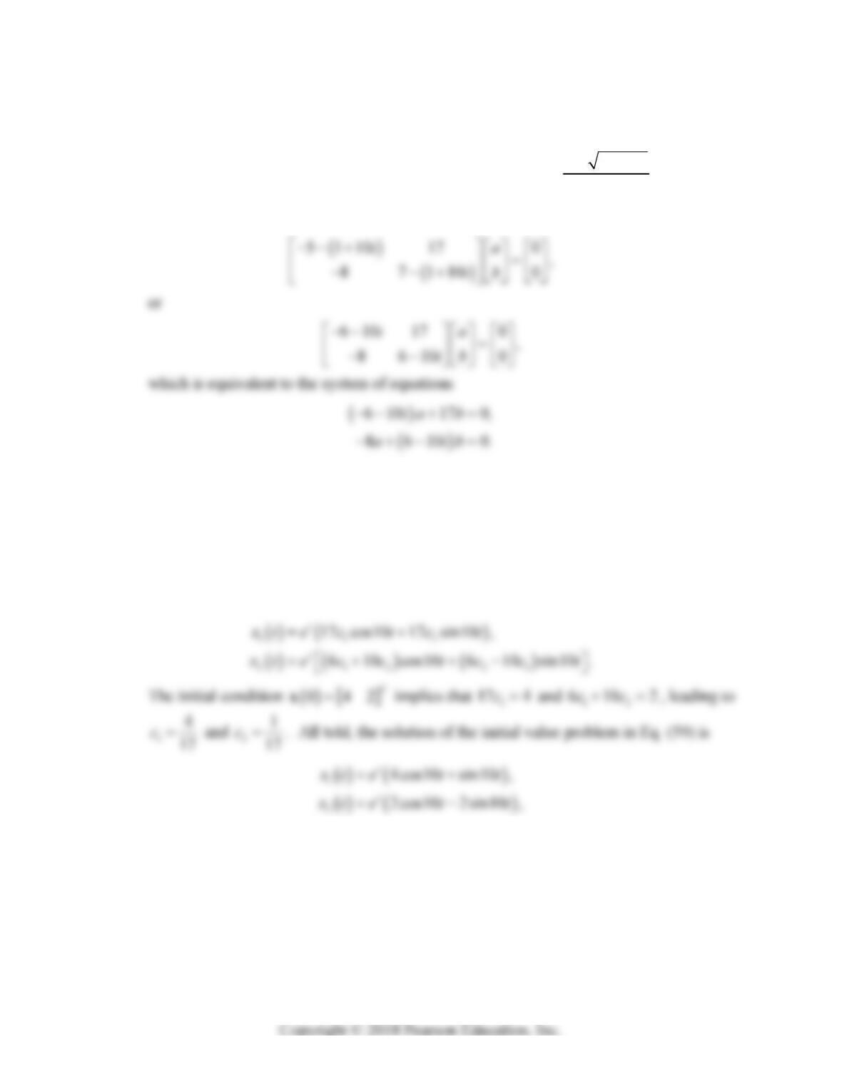
39. a) The characteristic equation of A is given by
det 0
AI , that is
20
ab
a d bc a d ad bc
cd
.
432 Chapter 7: Linear Systems of Differential Equations
40. From the result of Problem 39, the characteristic equation of the matrix 517
87
A is
22 101 0
, whose roots (the eigenvalues of A) are 2 4 404 110
2
i
.
An eigenvector
T
abv of A corresponding to 110i
satisfies
AIv0, or
Both of these equations are satisfied if 17a and 610bi , and so we can take
17 6 10 T
iv, with real and imaginary parts
17 6 T
a and
010
T
b. Thus
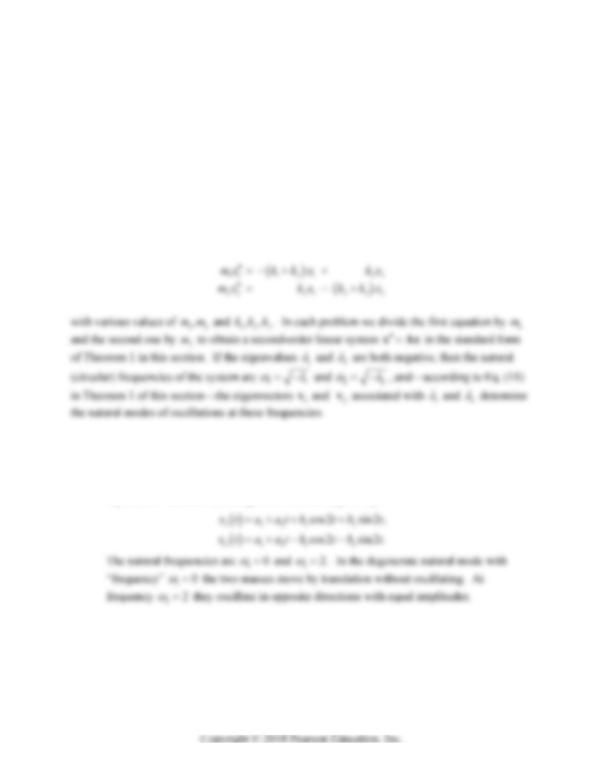
by Eq. (5) of this Section, the general solution of the system xAx is given by
12
17 0 0 17
cos10 sin10 cos10 sin10
610 106
tt
tce t tce t t
x,
or in scalar form,
in agreement with Eq. (61).
Section 7.5: Second-Order Systems and Mechanical Applications 433
SECTION 7.5
SECOND-ORDER SYSTEMS
AND MECHANICAL APPLICATIONS
This section uses the eigenvalue method to exhibit realistic applications of linear systems. If a
computer system like Maple, Mathematica, MATLAB, or even a TI calculator is available, then
a system of more than three railway cars, or a multistory building with four or more floors (as in
the project), can be investigated. However, the problems in the text are intended for manual
solution.
Problems 1–7 involve the system
1. The matrix 22
22
A has eigenvalues 00
and 14
with associated
eigenvectors
T
011v and
T
111v. Thus we have the special case described in
Eq. (12) of Theorem 1, and a general solution is given by
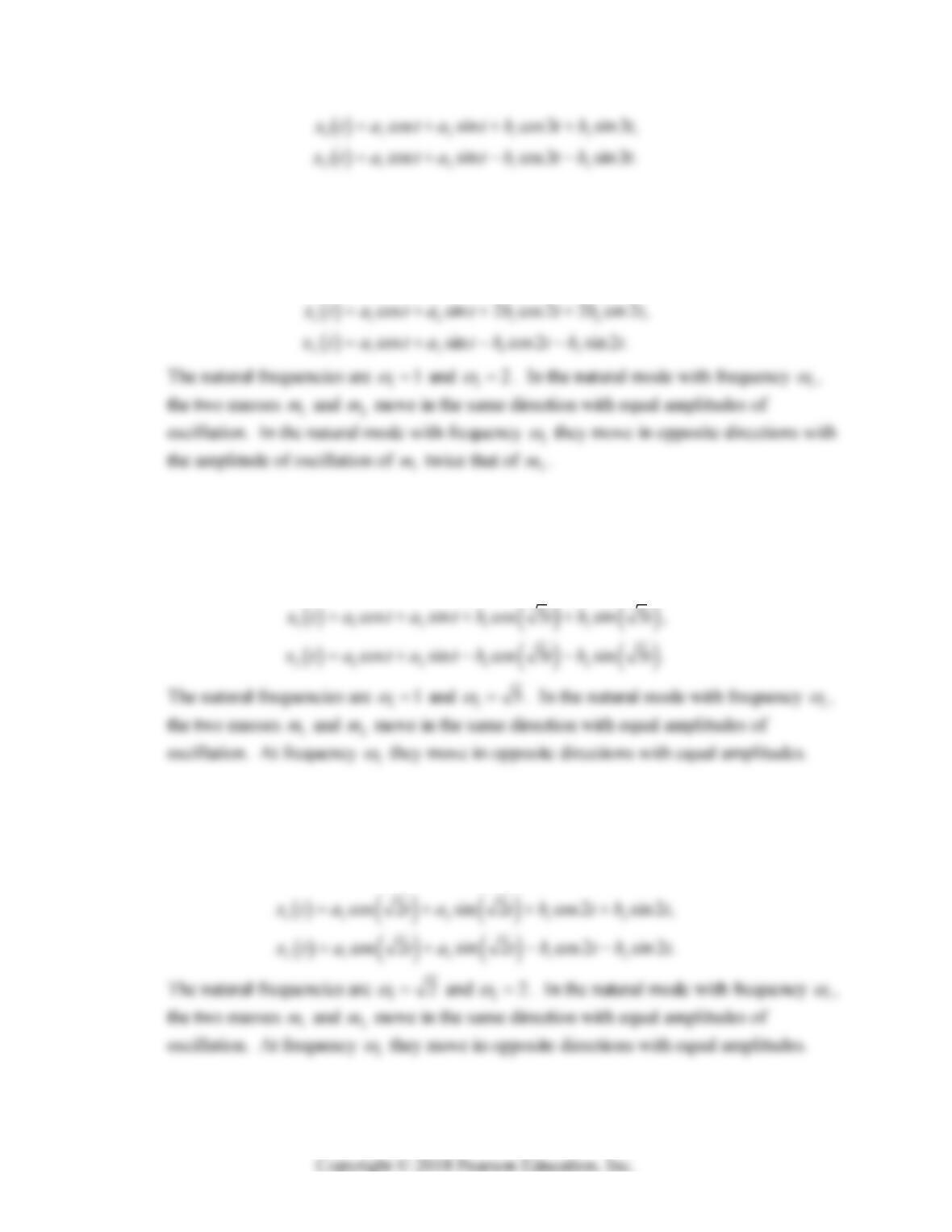
2. The matrix 54
55
A has eigenvalues 11
and 29
with associated
eigenvectors
T
111v and
T
211v. Hence a general solution is given by
434 Chapter 7: Linear Systems of Differential Equations
3. The matrix 32
12
A has eigenvalues 11
and 24
, with associated
eigenvectors
T
111v and
T
221v. Hence a general solution is given by
4. The matrix 32
23
A has eigenvalues 11
and 25
with associated
eigenvectors
T
111v and
T
211v. Hence a general solution is given by
5. The matrix 31
13
A has eigenvalues 12
and 24
with associated
eigenvectors
T
111v and
T
211v. Hence a general solution is given by