Section 5.3: Homogeneous Equations with Constant Coefficients 295
38. Given that 5r is one characteristic root, we divide 5r into the characteristic poly-
nomial 32
5 100 500rr r and get the remaining factor 2100r. Thus the general so-
39. The characteristic polynomial is
332
26128rrrr
, so the differential equation
is 6 12 8 0yy yy
.
42. The characteristic polynomial is
3
2642
4124864rrrr , so the differential
equation is (6) (4)
12 48 64 0yyyy
.
43. (a) Given a complex number zxiy we define r to be 22
x
y and
to bethe
x
44. (a)
242 1 3 ,2
22
ii
x
ii i
296 Chapter 5: Higher-Order Linear Differential Equations
45. The characteristic polynomial is the quadratic polynomial of Problem 44(b). Hence the
general solution is
47. The characteristic roots are
223 1 3rii , so the general solution is
13 13
12 1 2
cos 3 sin 3 cos 3 sin 3
ix ix xx
y x ce ce ce x i x ce x i x
.
48. The general solution is
x
xx
y x Ae Be Ce
, where 13
i
and
49. We adopt the same strategy as was used in Problem 48. The general solution is
2cos sin
xx
y
xAe Be C xDx
. Imposition of the given initial conditions yields
the equations
y
50. If 0x, then the differential equation is 0yy
, with general solution
cos sin
y
AxBx. But if 0x, then it is 0yy
, with general solution
Section 5.3: Homogeneous Equations with Constant Coefficients 297
y
y
51. In the solution of Problem 51 in Section 5.1 we showed that the substitution lnvx
gives 1dy dy
ydx x dv
and
22
22 22
11dy dy dy
ydx x dv x dv
. A further differentiation us-
ing the chain rule gives
52.
2
290
dy y
dv ; 290r; 3ri ;
121 2
cos3 sin 3 cos 3ln sin 3ln
y
xc vc vc xc x
298 Chapter 5: Higher-Order Linear Differential Equations
55.
32
32
440
dy dy dy
dv dv dv
; 32
440rrr; 0, 2, 2r;
22 2
12 3 1 23
ln
vv
y
xcce cve cxccx
3
58.
32
32
33 0
dy dy dy y
dv dv dv
; 32
3310rrr
; 1, 1, 1r ;
2
21
12 3 12 3
ln ln
vv v
y
xce cve cve xccxc x
SECTION 5.4
MECHANICAL VIBRATIONS
In this section we discuss four types of free motion of a mass on a spring—undamped, under-
damped, critically damped, and overdamped. However, the undamped and underdamped cas-
es—in which actual oscillations occur—are emphasized because they are both the most interest-
ing and the most important cases for applications.
1. Frequency: 0
16 1
2rad sec Hz
4
k
m
; period:
0
22 sec
2
P
Section 5.4: Mechanical Vibrations 299
4. (a) With 1kg
4
m and 9 N 0.25m=36 N mk , we find that 012 rad sec
. The solu-
tion of 144 0xx
with
01x and
05x is
5. The gravitational acceleration at distance R from the center of the earth is 2
GM
g
R
. Ac-
cording to Equation (6) in the text, the (circular) frequency
of a (linearized) pendulum
is given by 2
2
gGM
LRL
, so its period is 22L
pR
GM
.
6. If the pendulum in the clock executes n cycles per day (86400 sec) at Paris, then its peri-
od is 1
86400 secpn
. At the equatorial location it takes 24 hr 2 min 40sec 86560sec
R
p
p
7. The period equation
3960 100.10 3960 100px yields
1.9795mi 10.450ftx for the altitude of the mountain.
8. Let n be the number of cycles required for a correct clock with unknown pendulum
length 1
L and period 1
p
to register 24 hrs 86400sec, so 186400np . The given clock
p
300 Chapter 5: Higher-Order Linear Differential Equations
9. Designating
x
t as in the suggestion, we see that the mass is subject to a restorative
force
S
Fkx together with the force of gravity Wmg. We also assume that the
mass is subject to a damping force R
Fcx
. Applying Newton’s law then gives
y
x
x
x
10. The mass of the buoy is given by 2
mrh
, and the net downward force on the buoy is
22
Frhgrgx
. (Note that the depth
x
t is taken to be positive.) Therefore
Newton’s second law ma F gives
222
rh x rhg rg x
,
which simplifies to
g
x
xg
h
.
x
x
x
x
x
11. The differential equation from Problem 10 must be modified to reflect the fact that the
weight density of water is 3
62.4lb ft (as opposed to 3
1g cm
in the cgs system). Thus
Section 5.4: Mechanical Vibrations 301
ma F then gives 2
3.125 100 62.4
x
rx
, or 2
62.4 32
3.125
xrx
. The frequency
12. (a) Substitution of
3
r
r
M
M
R
in 2
r
r
GM m
Fr
yields 3
r
GMm
Fr
R
.
(b) Because 3
GM g
R
R
, the equation r
mr F
yields the differential equation
0
g
rr
R
.
(d) The orbital velocity v of such a satellite must be such that the centrifugal force
2
mv
R
on the satellite just offsets the weight mg of the satellite at the surface of the earth. Thus
2
mv mg
R, which implies that
244
32.2ft sec 3960 5280ft 2.5947 10 ft sec 1.7691 10 mi hrvgR .
302 Chapter 5: Higher-Order Linear Differential Equations
(e) The particle passes through the center of the earth when
0
cos 0rt R t
, that is,
when 02
t
, or
0
2
t
. At this time the speed of the particle is
4
00 0 0
0
sin sin 1.7691 10 mi hr
2
g
rt R t R R gR
R
.
13. (a) The characteristic equation
2
10 9 2 5 2 2 1 0rr r r has roots 21
,
52
r .
When we impose the initial conditions
00x,
05x on the general solution
25 2
12
tt
x
tce ce
we get the particular solution
25 2
50 tt
xt e e
.
14. (a) The characteristic equation
2
22
25 10 226 5 1 15 0rr r has roots
115 1 3
55
i
ri
. When we impose the initial conditions
020x,
041x on
the general solution
5cos3 sin 3
t
x
te A tB t
we get 20A, 15B. The corre-
Section 5.4: Mechanical Vibrations 303
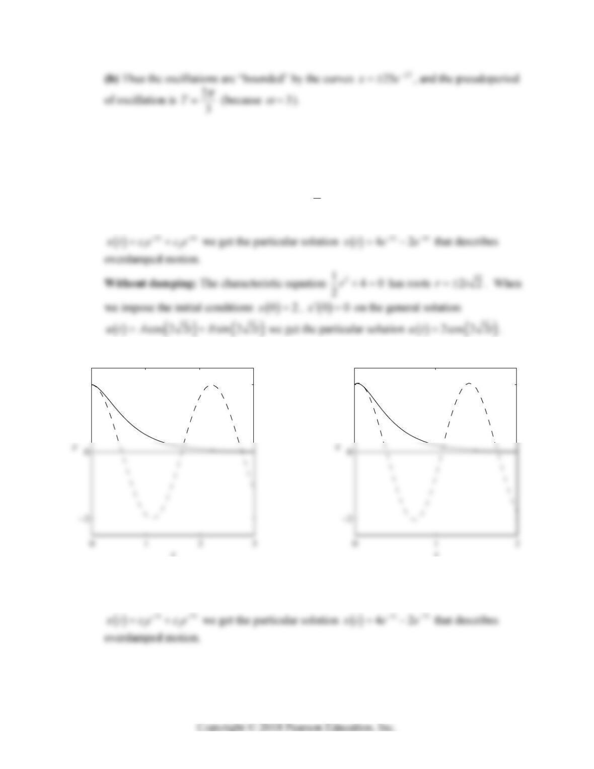
In Problems 15-21 the graph of the damped motion
x
t, that is, with the dashpot attached, is
shown as a solid line; the graph of the corresponding undamped motion
ut is dashed.
15. With damping: The characteristic equation 2
1340
2rr has roots 2, 4r . When
we impose the initial conditions
02x,
00x on the general solution
x
x
2
t
Problem 15
2
t
Problem 16
16. With damping: The characteristic equation 2
330630rr has roots 3, 7r .
When we impose the initial conditions
02x,
02x on the general solution
x
x
304 Chapter 5: Higher-Order Linear Differential Equations
17. With damping: The characteristic equation 28160rr has roots 4, 4r . When
we impose the initial conditions
05x,
010x on the general solution
4
12
t
x
tccte
we get the particular solution
4
521
t
xt e t
that describes crit-
ically damped motion.
5
t
Problem 17
1
t
Problem 18
18. With damping: The characteristic equation 2
212500rr
has roots 34ri .
When we impose the initial conditions
00x,
08x on the general solution
3cos4 sin 4
t
x
teA tB t
we get the particular solution
Section 5.4: Mechanical Vibrations 305
Without damping: The characteristic equation 2
2500r has roots 5ri . When
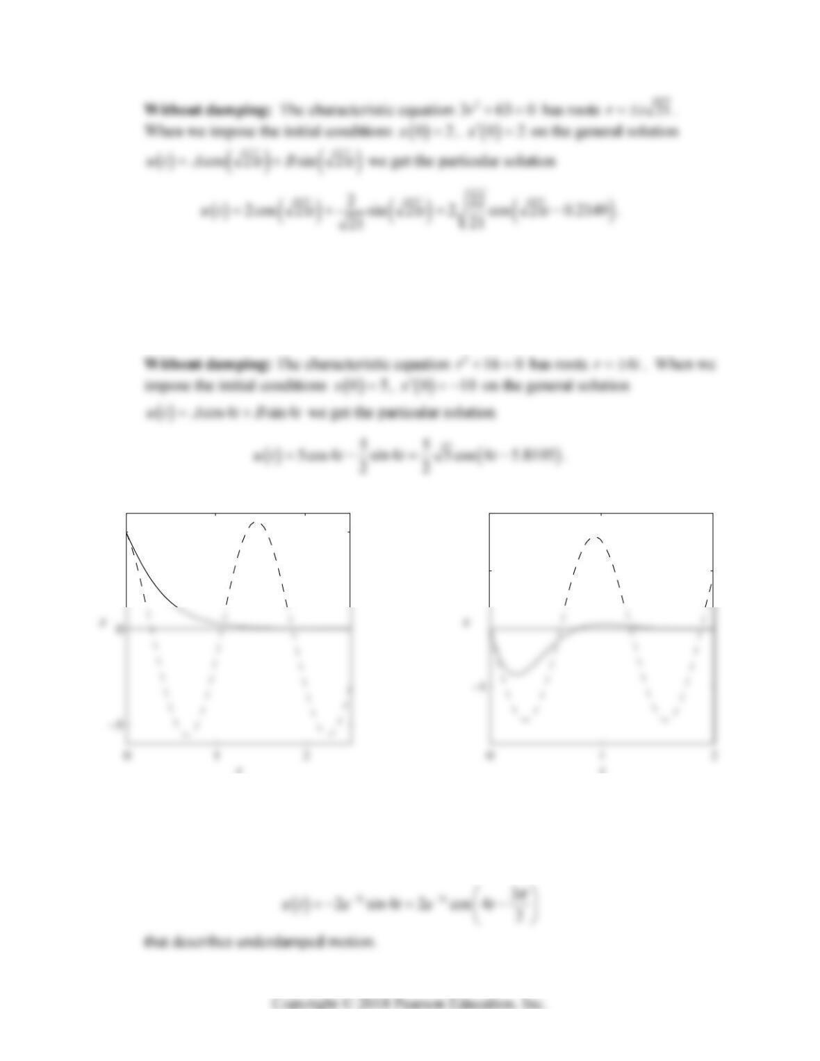
19. The characteristic equation 2
4 20 169 0rr has roots 56
2
ri . When we impose
the initial conditions
04x,
016x on the general solution
Without damping: The characteristic equation 2
4 169 0r has roots 13
2
ri . When
we impose the initial conditions
04x,
016x on the general solution
4
Problem 19
5
Problem 20
306 Chapter 5: Higher-Order Linear Differential Equations
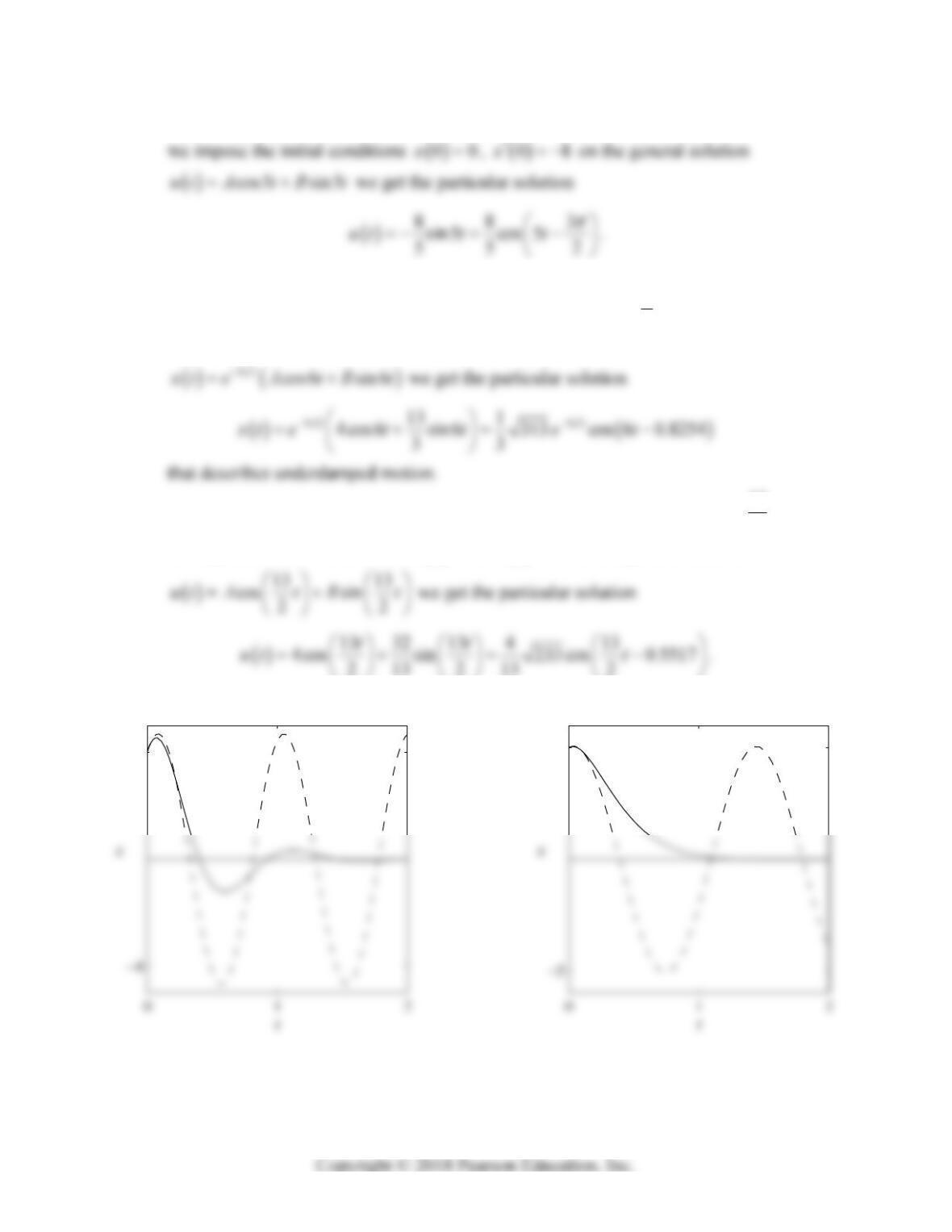
20. With damping: The characteristic equation 2
216400rr has roots 42ri .
When we impose the initial conditions
05x,
04x on the general solution
4cos2 sin 2
t
x
te A tB t
we get the particular solution
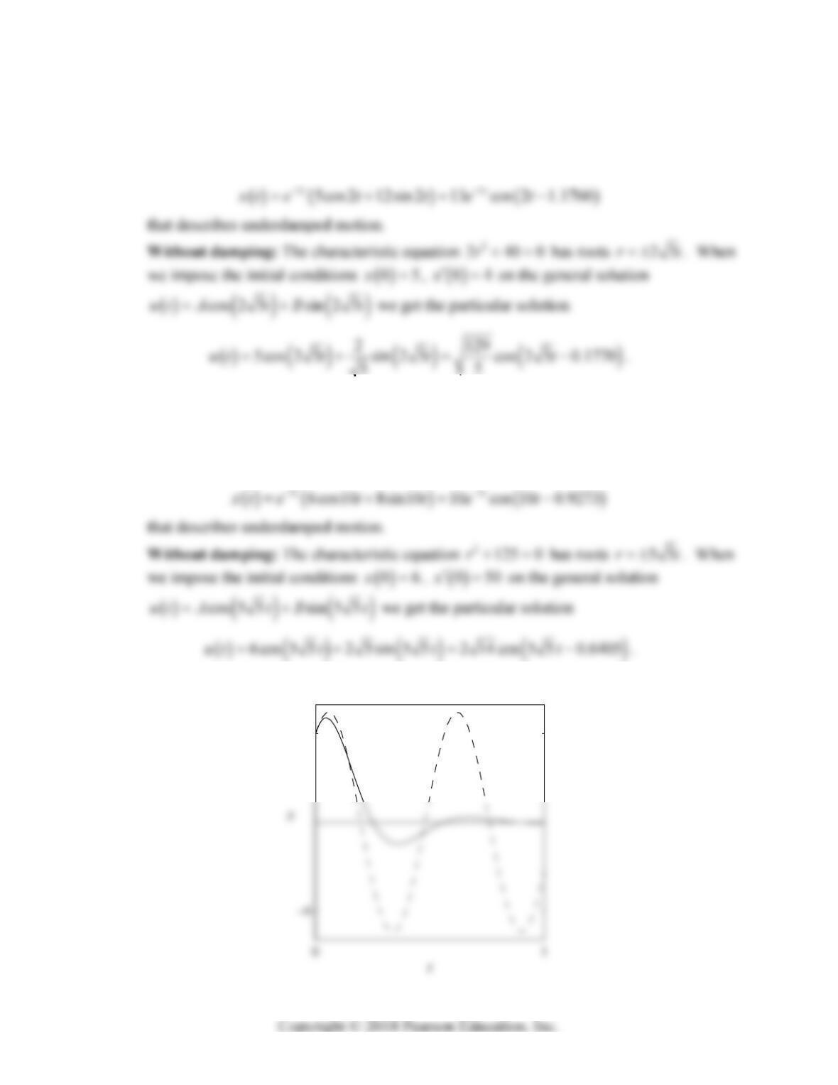
21. With damping: The characteristic equation 210 125 0rr has roots 510ri .
When we impose the initial conditions
06x,
050x on the general solution
5cos10 sin10
t
x
teA tB t
we get the particular solution
6
Problem 21
Section 5.4: Mechanical Vibrations 307
22. (a) With 12 0.375slug
32
m , 3lb–sec ftc, and 24lb ftk, the differential equation
is equivalent to 3 24 192 0xx x
. The characteristic equation 2
3 24 192 0rr
has roots 443ri . When we impose the initial conditions
01x,
00x on
the general solution
4cos 4 3 sin 4 3
t
x
te A tB t
we get the particular solu-
tion
23. (a) With 100slugm we get 100
k
. But we are given that
8
80cycles min 2 1min 60sec 3
,
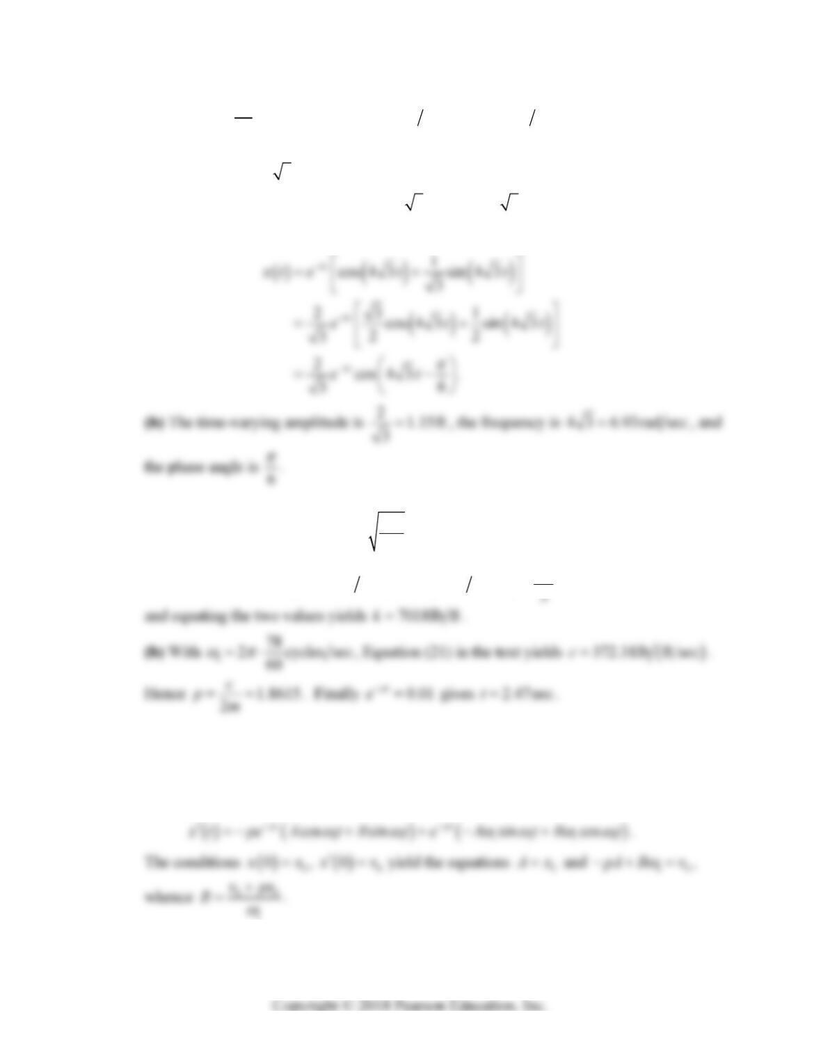
30. In the underdamped case we have
11
cos sin
pt
x
te A tB t
and
x
x
x
31. The binomial series
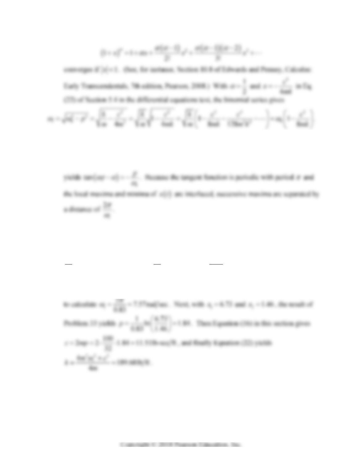
308 Chapter 5: Higher-Order Linear Differential Equations
32. If
1
cos
pt
xt Ce t
, then
111
cos sin 0
pt pt
xt pCe t C e t
x
33. If
11
x
xt and
22
x
xt are two successive local maxima, then 12 11 2tt
, and
so
1
111
cos
pt
xCe t
and
22
212 11
cos cos
pt pt
xCe t Ce t
. Hence
12
1
2
pt t
xe
x
and therefore
1
12
21
2
ln
x
p
pt t
x
.
34. With 10.34t and 21.17t we first use the equation 12 11 2tt
from Problem 33
35. The characteristic equation 2210rr
has roots 1, 1r . When we impose the ini-
tial conditions
00x,
10x on the general solution
12
t
x
tccte
we get the
particular solution
1
t
x
tte
.
Section 5.5: Nonhomogeneous Equations and Undetermined Coefficients 309
36. The characteristic equation
22
2110 0
n
rr
has roots 110
n
r
. When we
impose the initial conditions
00x,
10x on the general solution
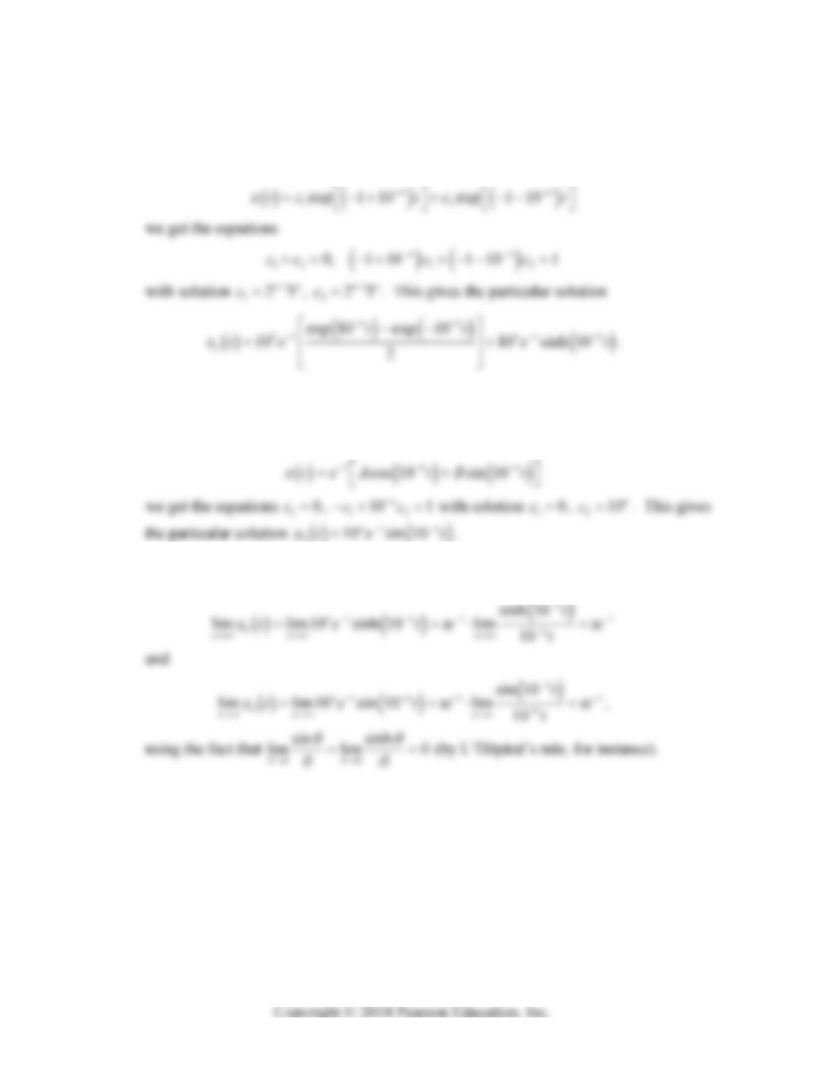
37. The characteristic equation
22
2110 0
n
rr
has roots 1 10 n
ri
. When we
impose the initial conditions
00x,
10x on the general solution
38. This follows from
SECTION 5.5
NONHOMOGENEOUS EQUATIONS AND UNDETERMINED
COEFFICIENTS
The method of undetermined coefficients is based on “educated guessing”. If we can guess cor-
rectly the form of a particular solution of a nonhomogeneous linear equation with constant coef-
ficients, then we can determine the particular solution explicitly by substitution in the given dif–
310 Chapter 5: Higher-Order Linear Differential Equations
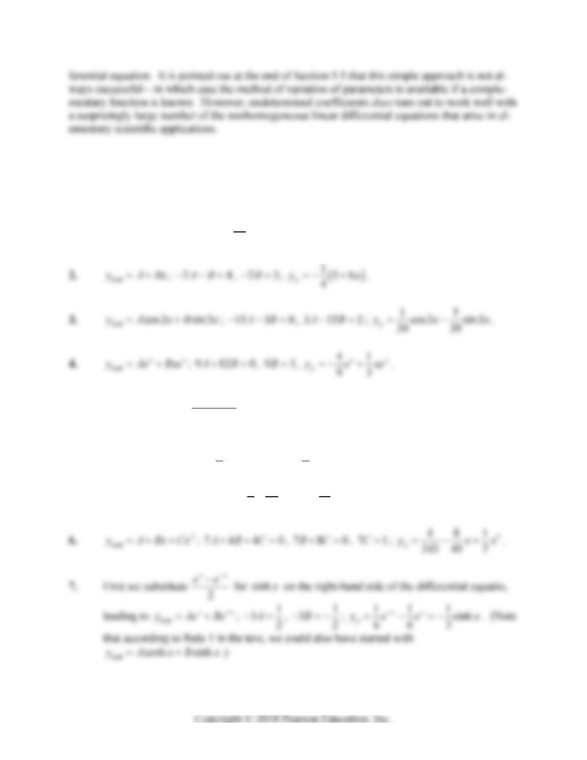
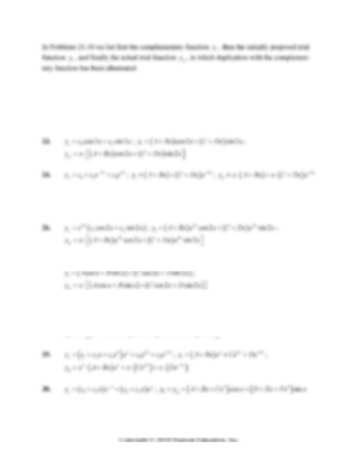
In each of Problems 1-20 we give first the form of the trial solution trial
y
, then the equations in
the coefficients we get when we substitute trial
y
into the differential equation and collect like
terms, and finally the resulting particular solution p
y
.
1. 3
trial
x
yAe; 25 1A; 3
1
25
x
p
ye.
y
y
y
x
x
5. First we substitute 1cos2
2
x
for 2
sin
x
on the right-hand side of the differential equa-
tion, leading to trial cos2 sin 2
y
AB xC x , and then
11
,32 ,23 0
22
ABC BC;
13 1
cos2 sin 2
226 13
p
yxx .
x
y
y
y
Section 5.5: Nonhomogeneous Equations and Undetermined Coefficients 311
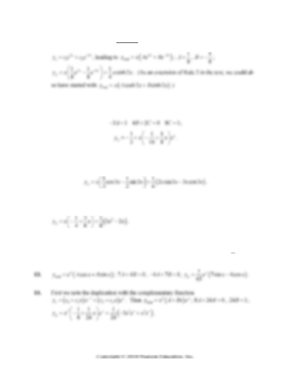
8. First we note that
22
cosh 2 2
x
x
ee
x
is part of the complementary function
x
y
y
9. First we note that
x
e is part of the complementary function 3
12
x
x
c
ycece
. Then
trial
x
yAxBCxe , and then
x
y
10. First we note the duplication with the complementary function 12
cos3 sin 3
c
y
cxcx.
Then
trial cos3 sin 3yxAxBx; 62B; 63A;
y
11. First we note the duplication with the complementary function
12 3
cos 2 sin 2
c
y
cc xc x . Then
trial
yxABx; 4 1A , 83B;
y
12. First we note the duplication with the complementary function 12 3
cos sin
c
y
cc xc x .
Then
trial cos sinyAxxBxCx ; 2A, 20B, 21C; 1
2sin
2
p
yxxx .
x
x
x
y
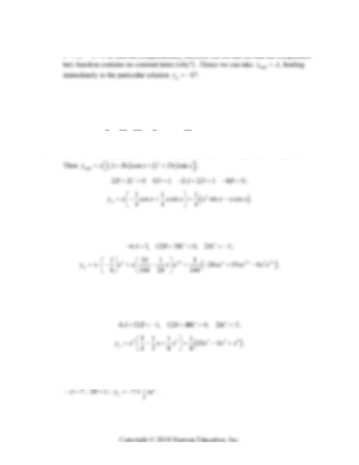
312 Chapter 5: Higher-Order Linear Differential Equations
15. This is something of a trick problem. We cannot solve the characteristic equation
54
y
16.
23
trial
x
yABCxDxe ;
95,18620,18120,182ABCDCD D ;
23 3 3 23
512 1 1
45 6 9
98127 9 81
x
xx x
p
y
xxe e xe xe
.
17. First we note the duplication with the complementary function 12
cos sin
c
y
cxcx.
y
y
18. First we note the duplication with the complementary function
22
123 4
x
xxx
c
yce cece ce
. Then
2
trial
x
x
yxAexBCxe ;
x
y
19. First we note the duplication with the part 12
ccx of the complementary function (which
corresponds to the factor 2
r of the characteristic polynomial). Then
22
trial
y
xABxCx;
y
20. First we note that the characteristic polynomial 3
rr has the zero 1r corresponding to
the duplicating part
x
e of the complementary function. Then: trial
x
y
AxBe ;
x
Section 5.5: Nonhomogeneous Equations and Undetermined Coefficients 313
y
y
y
21.
c1 2
cos sin
x
yec xc x;
icos sin
x
yeA xB x;
cos sin
x
p
yxeAxBx
22.
2
12 3 4 5
x
x
c
y
ccxcx ce ce
;
2
i
x
y
ABxCx De ;
32
x
p
yxABxCx xDe
y
x
x
x
25. 2
12
x
x
c
yce ce
;
2
i
x
x
yABxe CDxe
;
2
x
x
p
yxABxe xCDxe
27.
12 3 4
cos sin cos2 sin 2
c
ycxcxc xc x ;
y
28.
12 3 4
cos3 sin 3
c
yccxc xc x ;
22
icos3 sin 3
y
ABxCx x DExFx x ;
22
cos3 sin 3
x
x
x
x
y
y
x A Bx Cx x D Ex Fx x
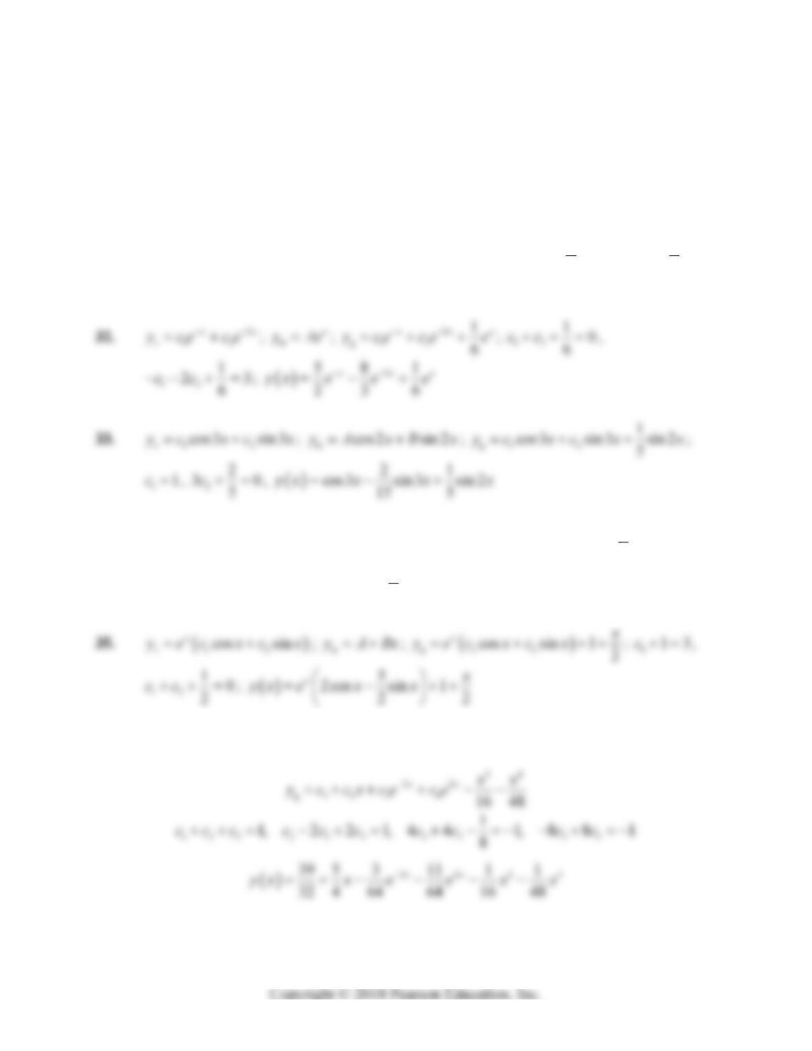
314 Chapter 5: Higher-Order Linear Differential Equations
In Problems 31-40 we list first the complementary function c
y
, the trial solution tr
y
for the
method of undetermined coefficients, and the corresponding general solution gcp
y
yy,
where p
y results from determining the coefficients in tr
y
so as to satisfy the given nonhomoge-
neous differential equation. Then we list the linear equations obtained by imposing the given
initial conditions, and finally the resulting particular solution
yx.
31. 12
cos2 sin 2
c
y
cxcx; tr
y
ABx ; g1 2
cos2 sin 2 2
x
yc xc x
;11c, 2
1
22
2
c
;
() cos2 (3/4)sin2 /2
y
xx xx
y
y
y
y
y
34. 12
cos sin
c
y
cxcx;
tr cos sinyxAxBx ; g1 2
1
cos sin sin
2
yc xc x xx ;
11c, 21c ,
1
cos sin sin
2
yx x x x x
y
x
x
36. 22
12 3 4
x
x
c
y
ccxce ce
;
22
tr
yxABxCx
x