Section 2.3: Acceleration-Velocity Models 135
the parachute opens, the initial value problem becomes 2
32 0.075vv
,
0 206.521v , with
0 4727.30y. Solving gives
24. Let M denote the mass of the Earth. Then
25. (a) The rocket’s apex occurs when 0v. We get the desired formula when we set 0v
in Eq. (23), 22
0
11
2vv GM
rR
, and solve for r.
26. By an elementary computation (as in Section 1.2) we find that an initial velocity of
016v ft/sec is required to jump vertically 4 feet high on earth. We must determine
whether this initial velocity is adequate for escape from the asteroid. Let r denote the
ratio of the radius of the asteroid to the radius 3960R miles of the earth, so that
a
136 Chapter 2: Mathematical Models and Numerical Methods
27. (a) Substitution of
2
2
0
2GM k
v
R
R
in Eq. (23) of the textbook gives
2dr GM k
v
dt r r
.
(b) If 0
2GM
v
R
, then Eq. (23) gives
28. (a) We proceed as in Example 4: Since dr
vdt
, dv
dt can be written as dv
vdr . Hence the
given differential equation 2
dv GM
dt r
becomes the separable equation 2
dv GM
vdr r
.
Separating variables gives 2
1
vdv GM dr
r
, and then integration gives
Section 2.3: Acceleration-Velocity Models 137
which under the substitution 2
0cosrr
becomes
29. Integration of 2
()
dv GM
vdy y R
,
00y,
0
0vv gives
30. When we integrate
2
2
em
dv GM GM
vdr r Sr
,
0rR,
0
0rv
in the usual way and
solve for v, we get
138 Chapter 2: Mathematical Models and Numerical Methods
SECTION 2.4
NUMERICAL APPROXIMATION: EULER’S METHOD
In each of Problems 1–10 we also give first the explicit form of Euler’s iterative formula for the
given differential equation ( , )
y
fxy
. As we illustrate in Problem 1, the desired iterations are
1. For the differential equation ( , )
y
fxy
with ( , )
f
xy y , the iterative formula of
Euler’s method is
1nn n
yyhy
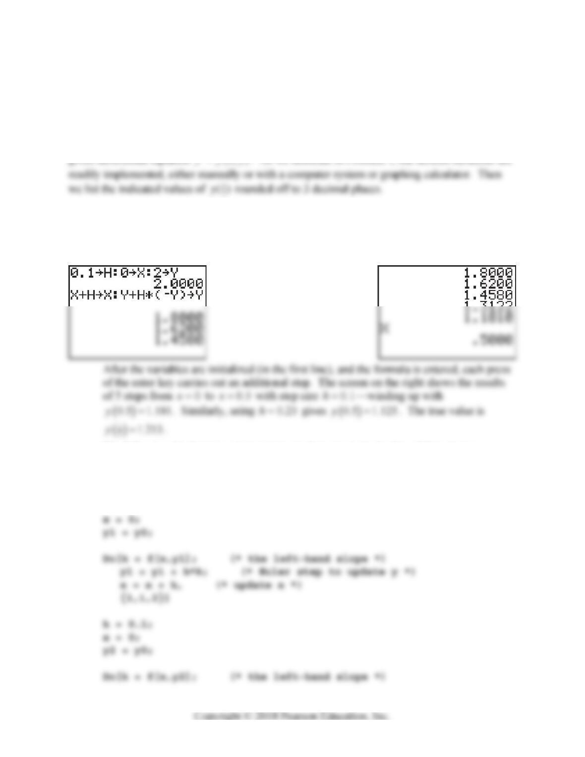
. The TI-83 screen on the left shows a graphing
calculator implementation of this iterative formula.
The following Mathematica instructions produce precisely the line of data shown:
f[x_,y_] = -y;
g[x_] = 2*Exp[-x];
y0 = 2;
h = 0.25;
Section 2.4: Numerical Approximation: Euler’s Method 139
2. Iterative formula:
12
nn n
yyhy
; approximate values 1.125 and 1.244; true value
1
21.359y.
3. Iterative formula:
11
nn n
yyhy
; approximate values 2.125 and 2.221; true value
1
22.297y.
6. Iterative formula:
12
nn nn
yyhxy
; approximate values 1.750 and 1.627; true value
1
21.558y.
7. Iterative formula:
2
13
nn nn
yyhxy
; approximate values 2.859 and 2.737; true value
1
22.647y.
10. Iterative formula:
2
12
nn nn
yyhxy
; approximate values 1.125 and 1.231; true value
1
21.333y.
140 Chapter 2: Mathematical Models and Numerical Methods
% Section 2.4, Problems 11-16
x0 = 0;
y0 = 1;
% first run:
% second run:
h = 0.005;
x = x0; y = y0; y2 = y0;
for n = 1:200
y = y + h*(y-2);
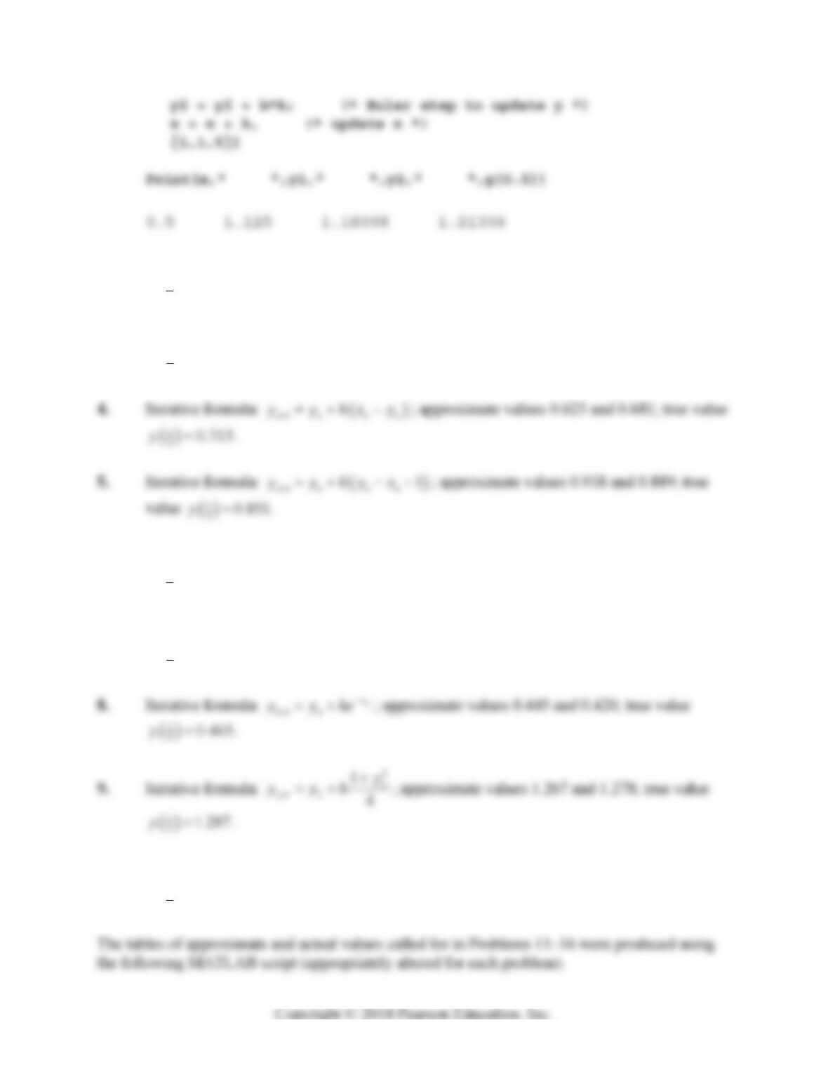
11. The iterative formula of Euler’s method is
12
nn n
yyhy
, and the exact solution is
2x
yx e . The resulting table of approximate and actual values is
x 0.0 0.2 0.4 0.6 0.8 1.0
y ( h = 0.01) 1.0000 0.7798 0.5111 0.1833 –0.2167 –0.7048
Section 2.4: Numerical Approximation: Euler’s Method 141
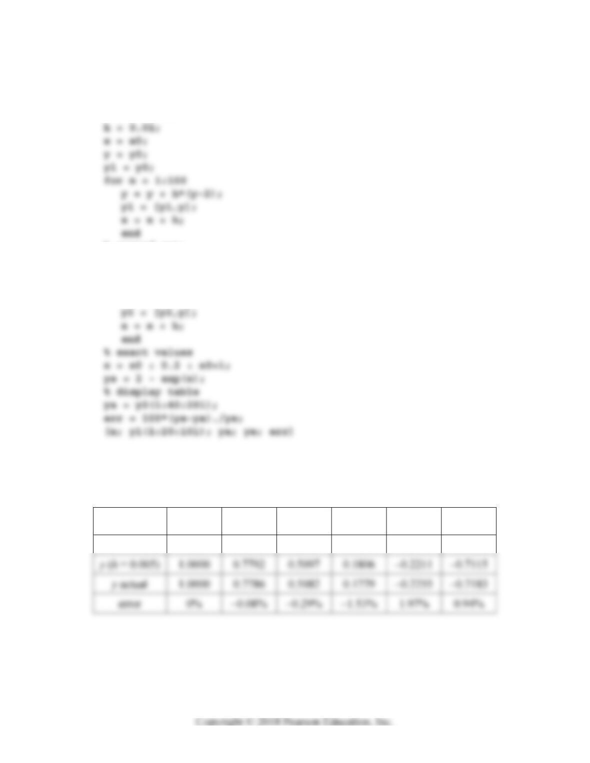
12. Iterative formula:
2
1
1
2
n
nn
y
yyh
; exact solution:
2
12
yx
x
.
x 0.0 0.2 0.4 0.6 0.8 1.0
y ( h=0.01) 2.0000 2.1105 2.2483 2.4250 2.6597 2.9864
13. Iterative formula:
3
12n
nn
n
x
yyh
y
; exact solution:
12
4
8yx x .
x 1.0 1.2 1.4 1.6 1.8 2.0
y ( h = 0.01) 3.0000 3.1718 3.4368 3.8084 4.2924 4.8890
14. Iterative formula:
2
1
n
nn
n
y
yyh
x
; exact solution:
1
1ln
yx
x
.
x 1.0 1.2 1.4 1.6 1.8 2.0
y ( h = 0.01) 1.0000 1.2215 1.5026 1.8761 2.4020 3.2031
142 Chapter 2: Mathematical Models and Numerical Methods
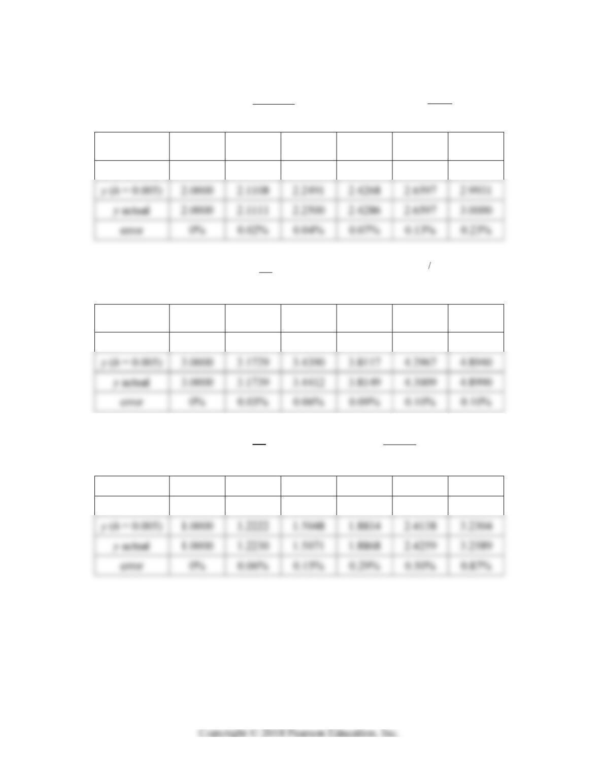
15. Iterative formula: 1
2
3n
nn
n
y
yyh
x
; exact solution:
2
4
yx x
x
.
x 2.0 2.2 2.4 2.6 2.8 3.0
y ( h = 0.01) 3.0000 3.0253 3.0927 3.1897 3.3080 3.4422
16. Iterative formula:
5
12
2n
nn
n
x
yyh
y
; exact solution:
13
637yx x .
x 2.0 2.2 2.4 2.6 2.8 3.0
y ( h = 0.01) 3.0000 4.2476 5.3650 6.4805 7.6343 8.8440
script similar to the one listed preceding the Problem 11 solution above.
17.
x 0.0 0.2 0.4 0.6 0.8 1.0
y ( h = 0.1) 0.0000 0.0010 0.0140 0.0551 0.1413 0.2925
Section 2.4: Numerical Approximation: Euler’s Method 143
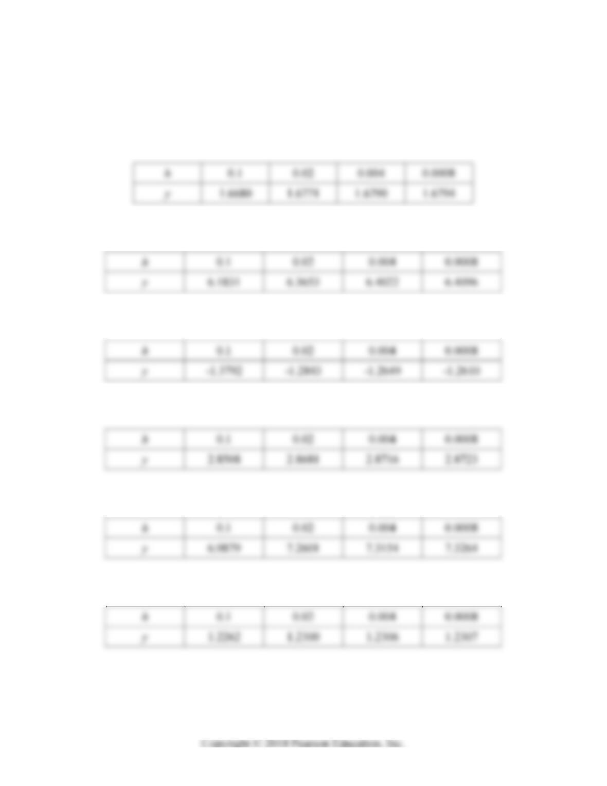
In Problems 1824 we give only the final approximate values of y obtained using Euler’s method
with step sizes 0.1h, 0.02h, 0.004h, and 0.0008h.
18. With 00x and 01y, the approximate values of
2y obtained are:
19. With 00x and 01y, the approximate values of
2y obtained are:
20. With 00x and 01y , the approximate values of
2y obtained are:
21. With 01x and 02y, the approximate values of
2y obtained are:
22. With 00x and 01y, the approximate values of
2y obtained are:
23. With 00x and 00y, the approximate values of
1y obtained are:
144 Chapter 2: Mathematical Models and Numerical Methods
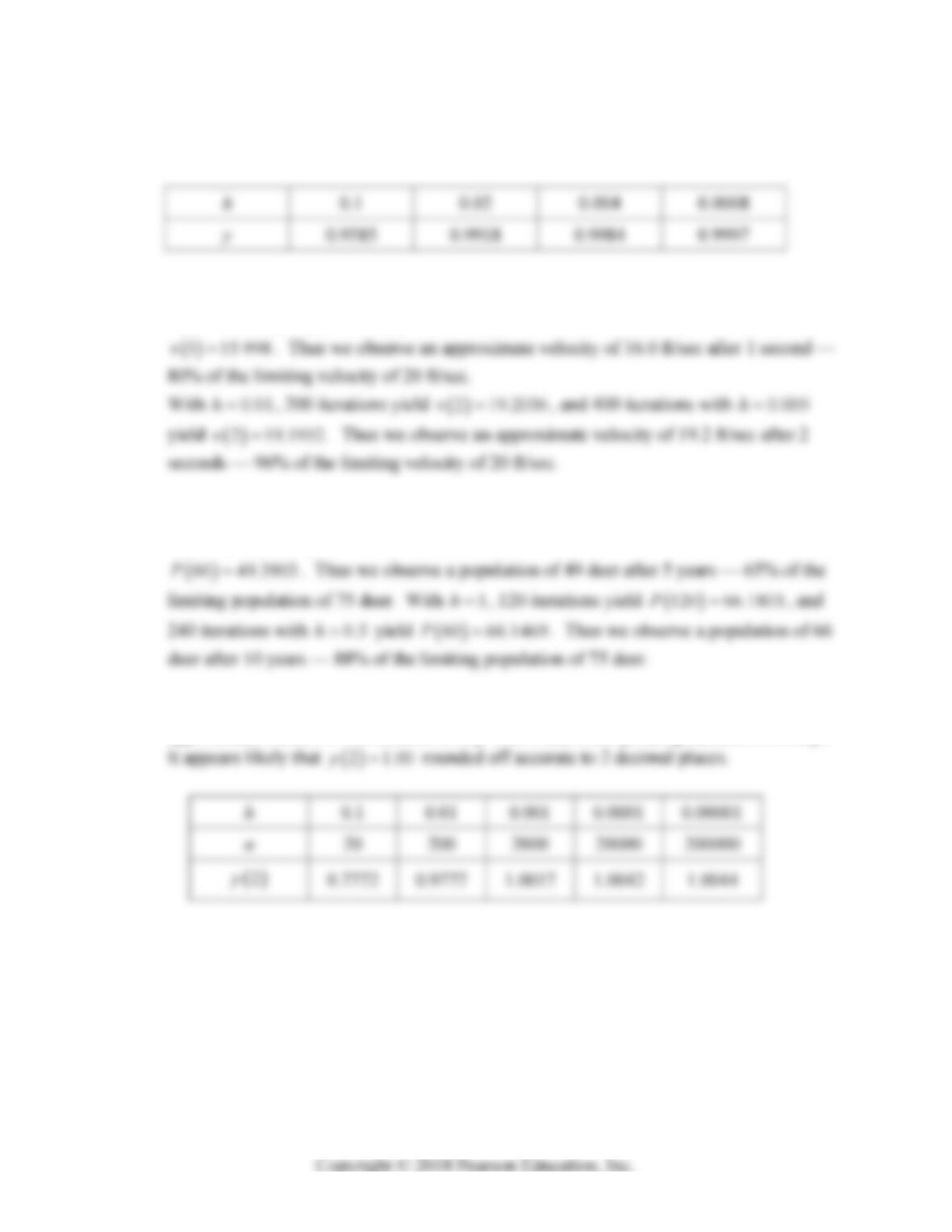
24. With 01x and 01y, the approximate values of
1y obtained are:
25. Here
,321.6
f
tv v and 00t, 00v. With 0.01h, 100 iterations of
1,
nn nn
vvhftv
yield
1 16.014v, and 200 iterations with 0.005h yield
26. Here
2
, 0.0225 0.003
f
tP P P
and 00t, 025P. With 1h, 60 iterations of
1,
nn nn
PPhftP
yield
60 49.3888P, and 120 iterations with 0.5h yield
27. Here
22
,1fxy x y
and 00x,00y. The following table gives the
approximate values for the successive step sizes h and corresponding numbers n of steps.
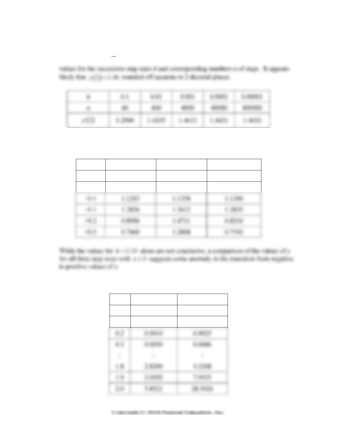
Section 2.4: Numerical Approximation: Euler’s Method 145
28. Here
2
1
,2
f
xy x y and 02x , 00y. The following table gives the approximate
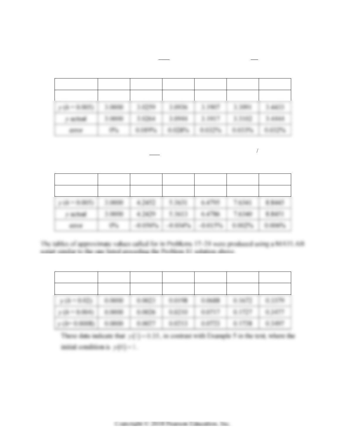
29. With step sizes 0.15h, 0.03h, and 0.006h, we get the following results:
x y with 0.15h y with 0.03h y with 0.006h
1.0 1.0000 1.0000 1.0000
0.7 1.0472 1.0512 1.0521
30. With step sizes 0.1h and 0.01h we get the following results:
x y with 0.1h y with 0.01h
0.0 0.0000 0.0000
0.1 0.0000 0.0003
146 Chapter 2: Mathematical Models and Numerical Methods
Clearly there is some difficulty near 2x.
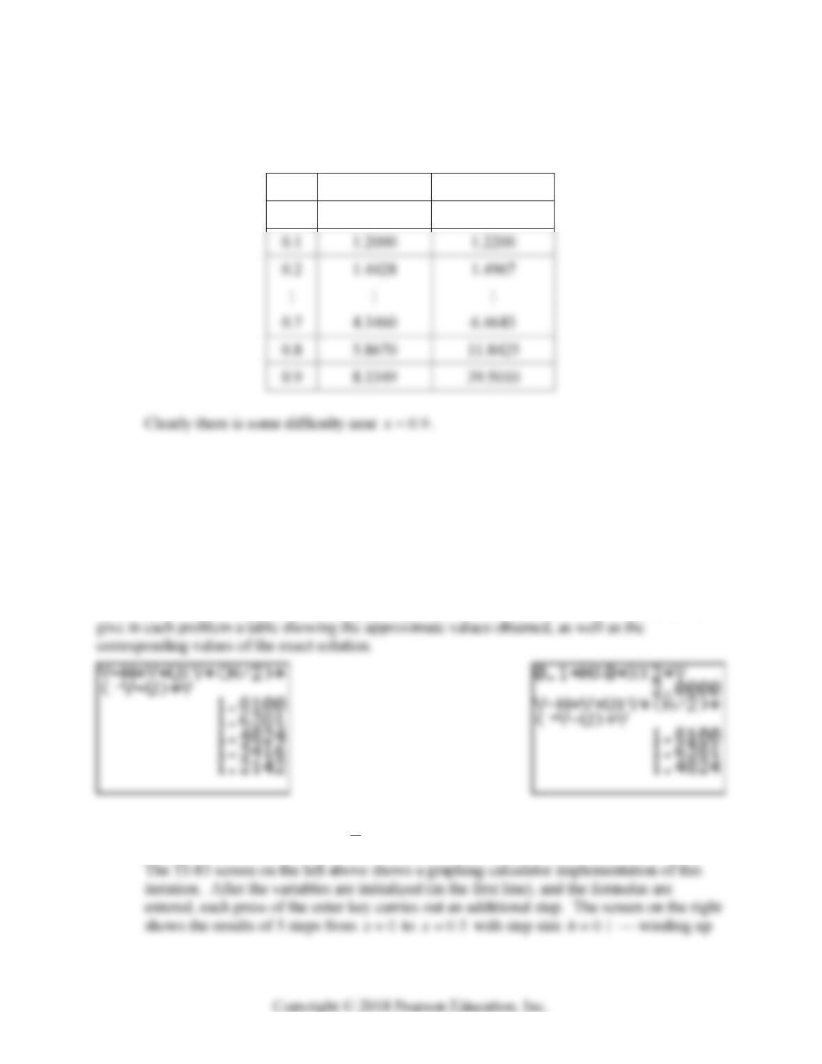
31. With step sizes h = 0.1 and h = 0.01 we get the following results:
x y with 0.1h y with 0.01h
0.0 1.0000 1.0000
SECTION 2.5
A CLOSER LOOK AT THE EULER METHOD
In each of Problems 1–10 we give first the predictor formula for 1n
u and then the improved
Euler corrector for 1n
y. These predictor-corrector iterations are readily implemented, either
manually or with a computer system or graphing calculator (as we illustrate in Problem 1). We
1.
1nn n
uyhy
;
11
2
nn nn
h
yy yu
Section 2.5: A Closer Look at the Euler Method 147
2. 12
nn n
uyhy
;
11
22
2
nn nn
h
yy yu
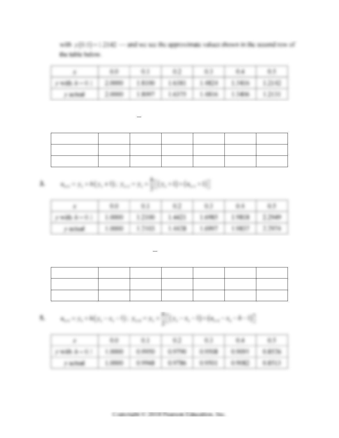
x 0.0 0.1 0.2 0.3 0.4 0.5
y with 0.1h 0.5000 0.6100 0.7422 0.9079 1.1077 1.3514
y actual 0.5000 0.6107 0.7459 0.9111 1.1128 1.3591
4.
1nn nn
uyhxy
;
11
2
nn nnn n
h
yy xyxhu
x 0.0 0.1 0.2 0.3 0.4 0.5
y with 0.1h 1.0000 0.9100 0.8381 0.7824 0.7416 0.7142
y actual 1.0000 0.9097 0.8375 0.7816 0.7406 0.7131
148 Chapter 2: Mathematical Models and Numerical Methods
6. 12
nnnn
uyxyh
;
11
22
2
nn nnnn
h
yy xy xhu
x 0.0 0.1 0.2 0.3 0.4 0.5
y with 0.1h 2.0000 1.9800 1.9214 1.8276 1.7041 1.5575
y actual 2.0000 1.9801 1.9216 1.8279 1.7043 1.5576
8. 1
n
y
nn
uyhe
; 1
12
nn
yu
nn
h
yy ee
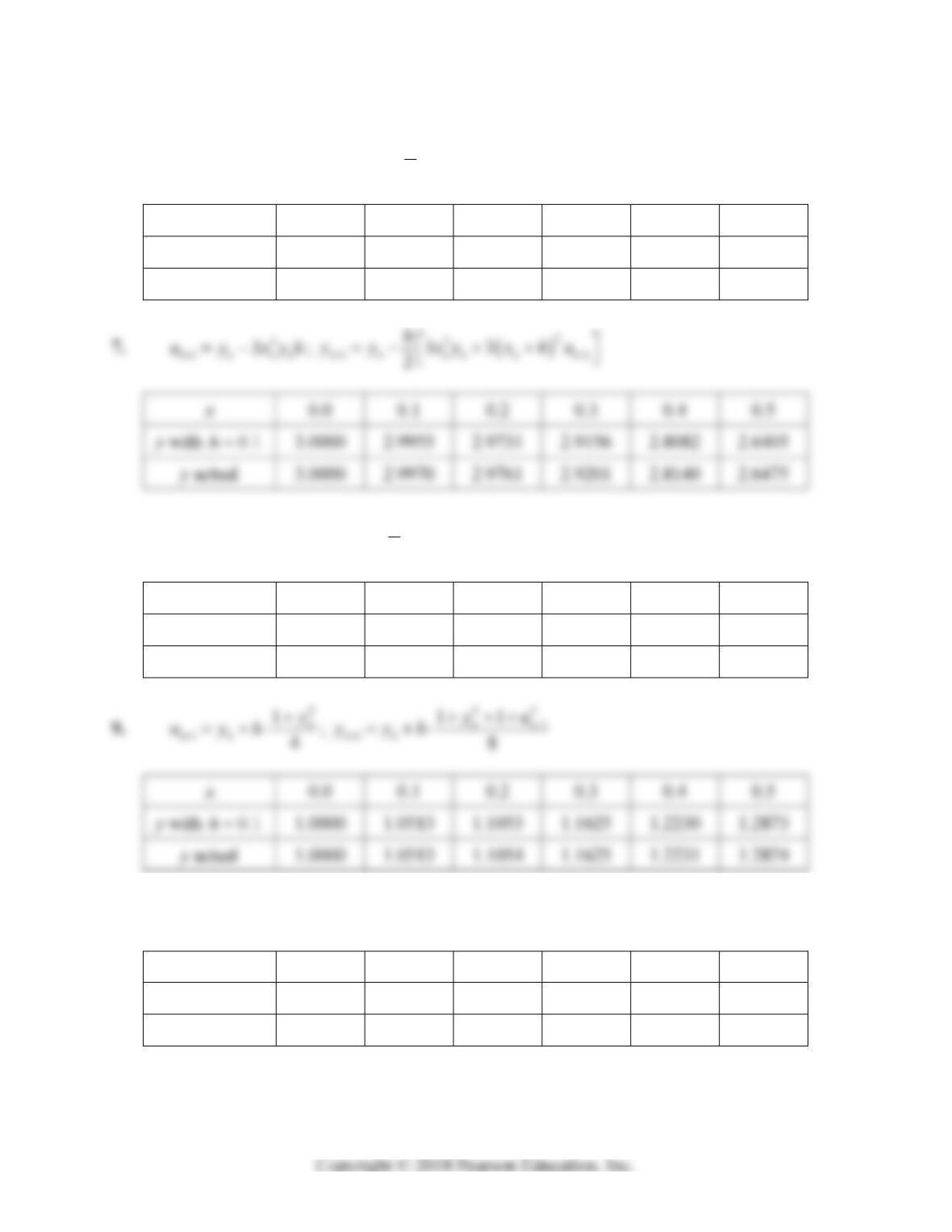
x 0.0 0.1 0.2 0.3 0.4 0.5
y with 0.1h 0.0000 0.0952 0.1822 0.2622 0.3363 0.4053
y actual 0.0000 0.0953 0.1823 0.2624 0.3365 0.4055
10. 2
12
nn nn
uyhxy
;
22
11nn nnn n
yyhxyxhu
x 0.0 0.1 0.2 0.3 0.4 0.5
y with 0.1h 1.0000 1.0100 1.0414 1.0984 1.1895 1.3309
y actual 1.0000 1.0101 1.0417 1.0989 1.1905 1.3333
Section 2.5: A Closer Look at the Euler Method 149
The results given below for Problems 11–16 were computed using the following MATLAB
script.
% Section 2.5, Problems 11-16
x0 = 0; y0 = 1;
% first run:
h = 0.01;
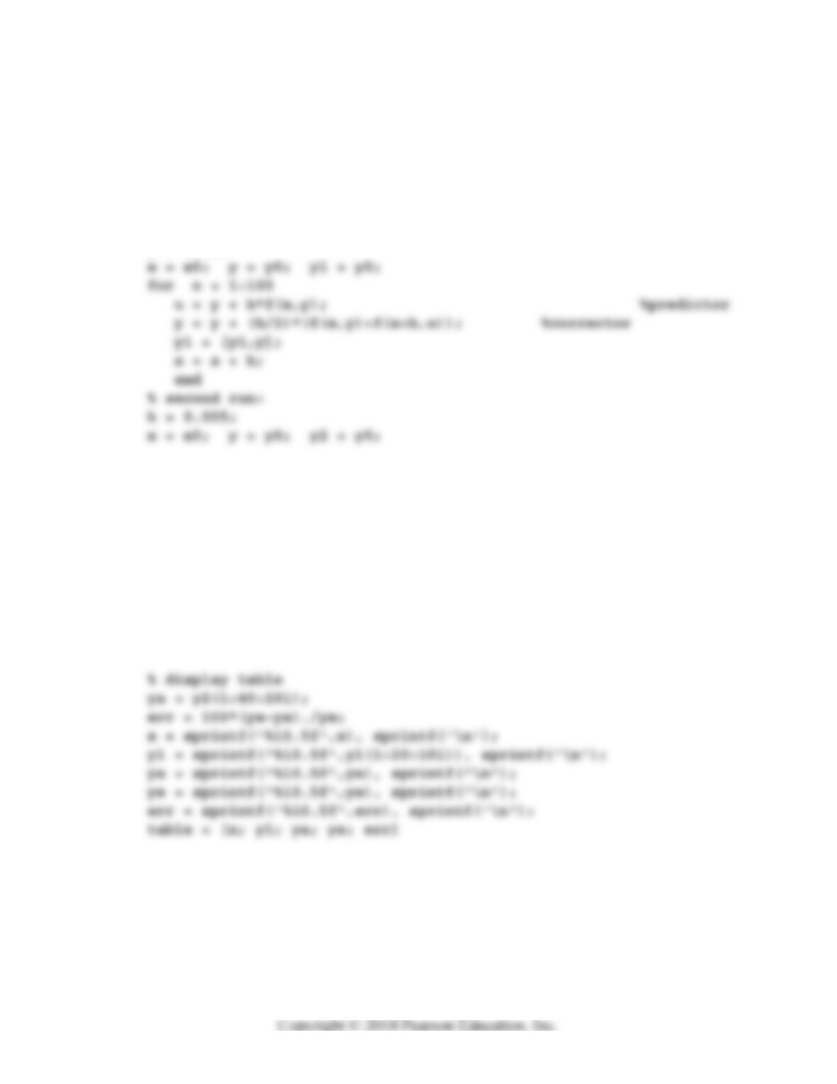
for n = 1:200
u = y + h*f(x,y); %predictor
y = y + (h/2)*(f(x,y)+f(x+h,u)); %corrector
y2 = [y2,y];
x = x + h;
end
% exact values
x = x0 : 0.2 : x0+1;
ye = g(x);
For each problem the differential equation ( , )
y
fxy
and the known exact solution
ygx
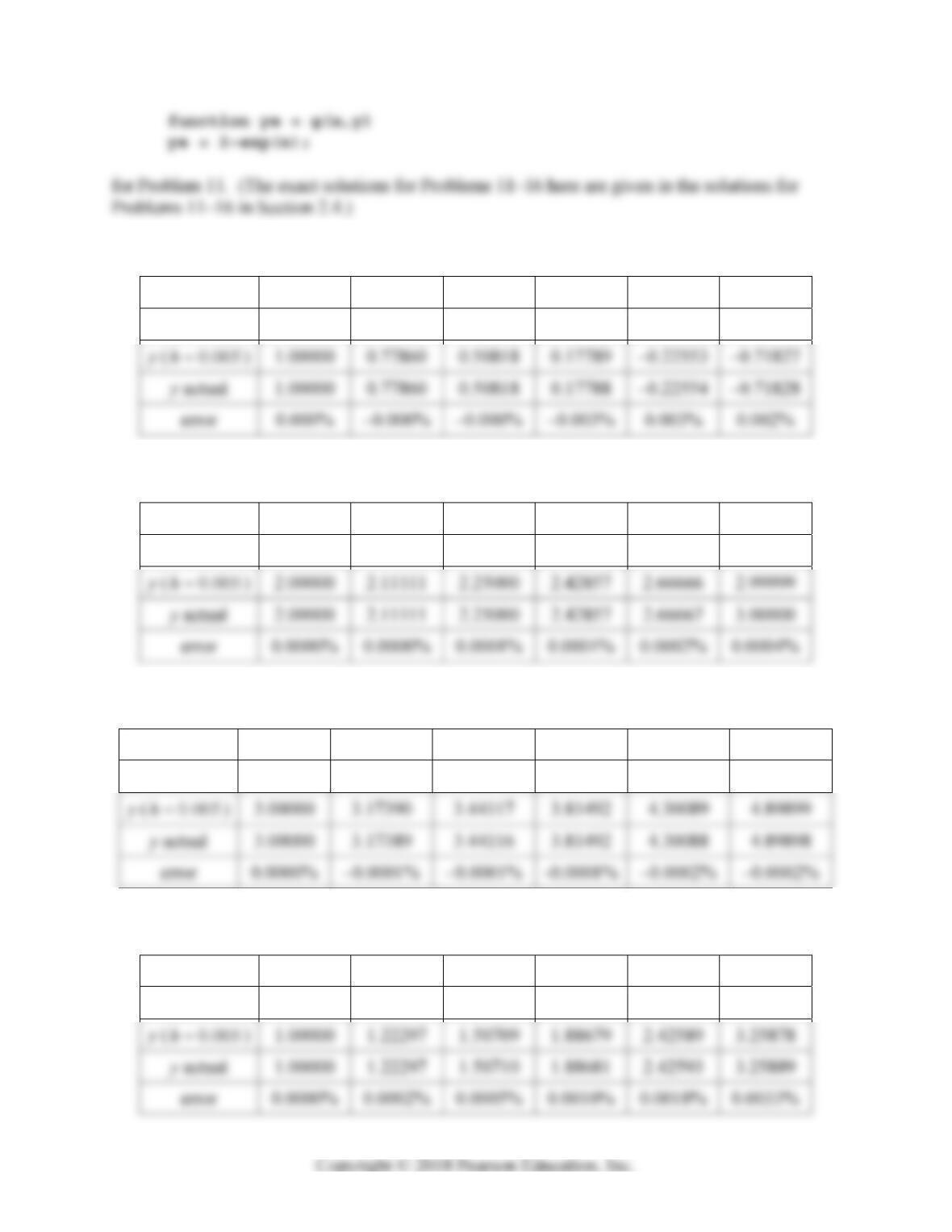
are stored in the files f.m and g.m — for instance, the files
function yp = f(x,y)
yp = y-2;
150 Chapter 2: Mathematical Models and Numerical Methods
11.
x 0.0 0.2 0.4 0.6 0.8 1.0
y ( 0.01h) 1.00000 0.77860 0.50819 0.17790 –0.22551 –0.71824
12.
x 0.0 0.2 0.4 0.6 0.8 1.0
y ( 0.01h) 2.00000 2.11111 2.25000 2.42856 2.66664 2.99995
13.
x 1.0 1.2 1.4 1.6 1.8 2.0
y ( 0.01h) 3.00000 3.17390 3.44118 3.81494 4.30091 4.89901
14.
x 1.0 1.2 1.4 1.6 1.8 2.0
y ( 0.01h) 1.00000 1.22296 1.50707 1.88673 2.42576 3.25847
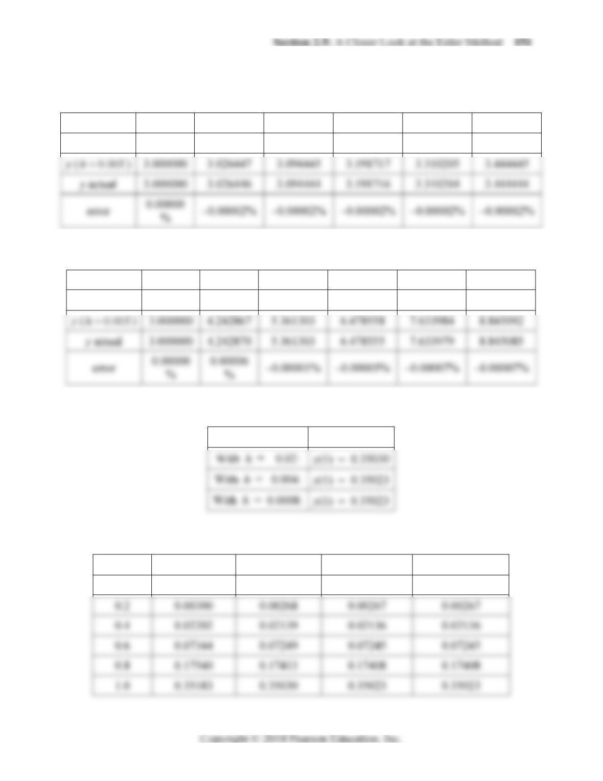
15.
x 2.0 2.2 2.4 2.6 2.8 3.0
y ( 0.01h) 3.000000 3.026448 3.094447 3.191719 3.310207 3.444448
16.
x 2.0 2.2 2.4 2.6 2.8 3.0
y ( 0.01h) 3.000000 4.242859 5.361304 6.478567 7.633999 8.845112
17.
With h = 0.1: y(1) 0.35183
The table of numerical results is
x y with 0.1h y with 0.02h y with 0.004h y with 0.0008h
0.0 0.00000 0.00000 0.00000 0.00000
152 Chapter 2: Mathematical Models and Numerical Methods
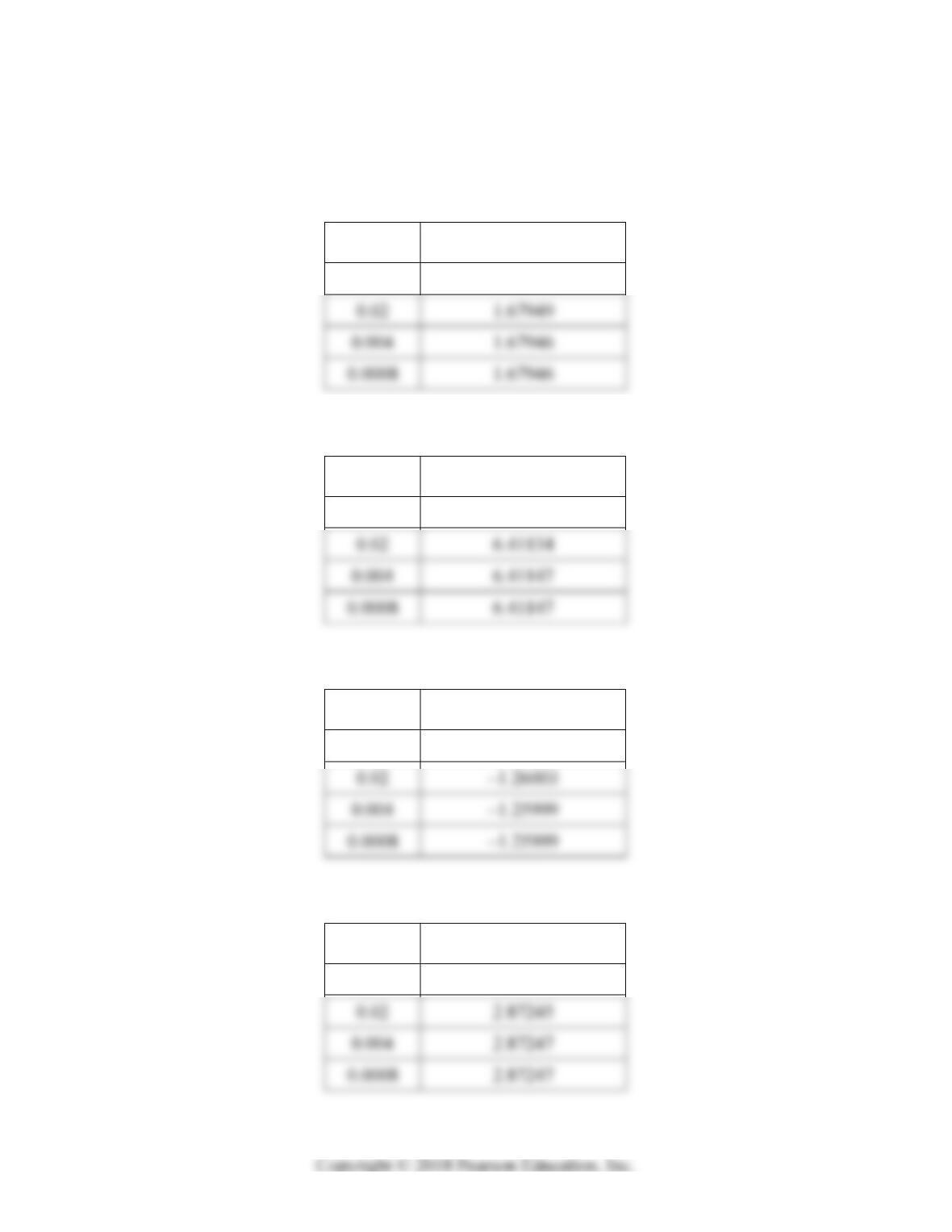
In Problems 1824 we give only the final approximate values of y obtained using the improved
Euler method with step sizes h = 0.1, h = 0.02, h = 0.004, and h = 0.0008.
18.
Value of h Estimated value of
2y
0.1 1.68043
19.
Value of h Estimated value of
2y
0.1 6.40834
20.
Value of h Estimated value of
2y
0.1 –1.26092
21.
Value of h Estimated value of
2y
0.1 2.87204
Section 2.5: A Closer Look at the Euler Method 153
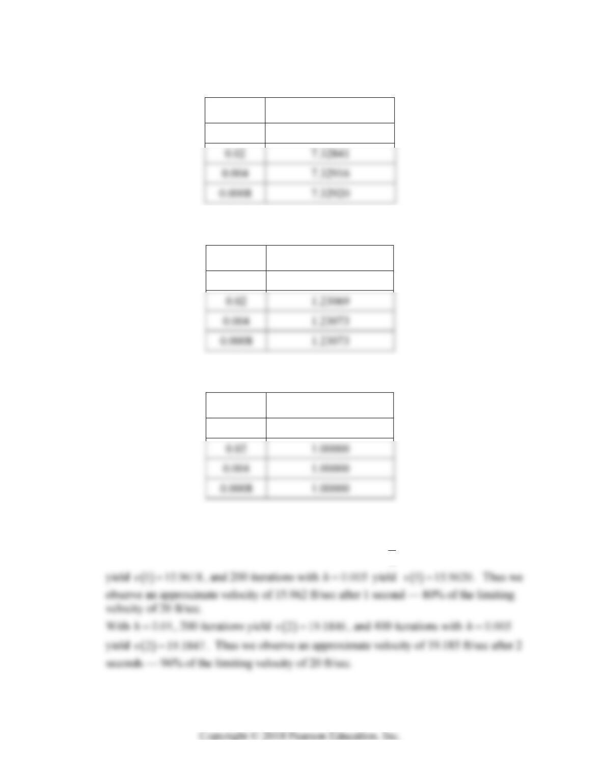
22.
Value of h Estimated value of
2y
0.1 7.31578
23.
Value of h Estimated value of
1y
0.1 1.22967
24.
Value of h Estimated value of
1y
0.1 1.00006
25. Here
,321.6
f
tv v and 00t, 00v. With 0.01h, 100 iterations of
1,n
kftv,
21
,n
kfthvhk ,
112
2
nn
h
vv kk
154 Chapter 2: Mathematical Models and Numerical Methods
26. Here
2
, 0.0225 0.003
f
tP P P
and 00t, 025P. With 1h, 60 iterations of
1,n
kftP,
21
,n
kfthPhk ,
112
2
nn
h
PP kk
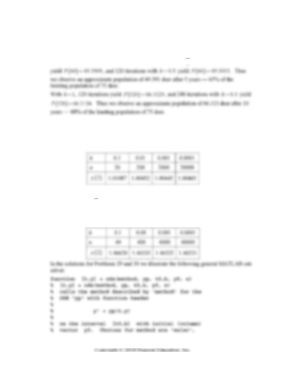
27. Here
22
,1fxy x y
and 00x, 00y. The following table gives the
approximate values for the successive step sizes h and corresponding numbers n of steps.
It appears likely that
2 1.0045y rounded off accurate to 4 decimal places.
28. Here
2
1
,2
f
xy x y and 02x , 00y. The following table gives the approximate
values for the successive step sizes h and corresponding numbers n of steps. It appears
likely that
2 1.4633y rounded off accurate to 4 decimal places.