Section 7.5: Second-Order Systems and Mechanical Applications 435
6. The matrix 64
24
A has eigenvalues 12
and 28
with associated
eigenvectors
T
111v and
T
221v. Hence a general solution is given by
7. The matrix 10 6
610
A has eigenvalues 14
and 216
with associated
eigenvectors
T
111v and
T
211v. Hence a general solution is given by
x
x
8. Substitution of the trial solution 11
cos5
x
ct, 22
cos5
x
ct in the system
112 212
54 96cos5, 45
x
xx tx xx
yields 15c and 21c, so a general solution is given by
x
x
x
x
436 Chapter 7: Linear Systems of Differential Equations
9. Substitution of the trial solution 11
cos3
x
ct, 22
cos3
x
ct in the system
112212
3 2 2 2 4 120cos3
x
xxx xx t
yields 13c and 29c , so a general solution is given by
x
x
x
x
10. Substitution of the trial solution 11
cos
x
ct, 22
cos
x
ct in the system
112 212
10 6 30cos , 6 10 60cos
x
xx tx x x t
yields 114c and 216c, so a general solution is given by
x
x
x
x
Section 7.5: Second-Order Systems and Mechanical Applications 437
11. (a) The matrix 40 8
12 60
A has eigenvalues 136
and 264
with associated
eigenvalues
T
121v and
T
213v. Hence a general solution is given by
x
y
(b) Substitution of the trial solution 1cos7
x
ct, 2cos7
y
ct in the system
40 8 195cos7 , 12 60 195cos7
x
xy ty x y t
yields 119c and 23c, so a general solution is given by
y
x
y
1212
2 cos6 2 sin 6 cos8 sin8 19 cos7 ,
x
ta ta tb tb t t
1
2
m;
in the same direction with frequency 37
and with the amplitude of motion of
1
m being 19
3 times that of 2
m.
438 Chapter 7: Linear Systems of Differential Equations
12. The coefficient matrix
21 0
121
01 2
A has characteristic polynomial
32 2
6104 2 42
.
13. The coefficient matrix
42 0
242
02 4
A has characteristic polynomial
32 2
12 40 32 4 8 8
.
14. The equations of motion of the given system are
1121
22 2 1
50 10 5cos10 ,
10 .
x
xxx t
mx x x
x
x
Section 7.5: Second-Order Systems and Mechanical Applications 439
15. First we need the general solution of the homogeneous system xAx with
50 25 2
50 50
A.
The eigenvalues of A are 125
and 275
, so the natural frequencies of the system
When we substitute the trial solution
T
12
cos10
ptcc tx in the nonhomogeneous
system, we find that 1
4
3
c and 2
16
3
c , so a particular solution
ptx is described by
12
416
cos10 , cos10
33
x
ttxt t
.
Finally, when we impose the zero initial conditions on the solution
cp
tttxx x
we find that 1
2
3
a, 20a, 12b , and 20b. Thus the solution we seek is described
by
x
x
16. The characteristic equation of A is
2
1212 12
0cccc cc
,
whence the given eigenvalues and eigenvectors follow readily.
440 Chapter 7: Linear Systems of Differential Equations
x
x
x
x
18. With 16c and 23c, it follows from Problem 16 that the natural frequencies and
associated eigenvectors are 10
,
T
111v and 23
,
T
221v. Hence
Theorem 1 gives the general solution
1112 2
2112 2
2cos3 2sin3,
cos3 sin 3 .
x
tabta tb t
x
tabta tb t
x
19. With 11c and 23c, it follows from Problem 16 that the natural frequencies and
associated eigenvectors are 10
,
T
111v and 22
,
T
213v. Hence
Theorem 1 gives the general solution
x
x
Section 7.5: Second-Order Systems and Mechanical Applications 441
The initial conditions
10
0
x
v
,
122
0000xxx
yield 12
0aa, 0
1
3
4
v
b,
and 0
28
v
b, so
The method of solution in each of Problems 20–23 is the same as that in Example 2 in this
section. Thus, looking at the equations in (26), we need to solve the equations
20. With
10
0
x
v
,
200x, and
30
0
x
v
, substitution of the resulting coefficient
values 123
,,bb b in (25) gives the railway car displacement functions
x
11
442 Chapter 7: Linear Systems of Differential Equations
21. With
10
02
x
v
,
200x, and
30
0
x
v
, substitution of the resulting coefficient
values 123
,,bb b in (25) gives the railway car displacement functions
x
x
x
We then see (substituting sin 4 2sin 2 cos 2ttt) that
21 0 0
11
sin 4 6sin 2 sin 2 cos 2 3
84
xt xt v t t v t t
remains negative until 2
t
(as does
32
x
txt, similarly) at which time the cars
separate with velocities
x
22. With
10
0
x
v
,
20
0
x
v
, and
30
02
x
v
, substitution of the resulting coefficient
values 123
,,bb b in (25) gives the railway car displacement functions
We then see (substituting sin 4 2sin 2 cos 2ttt) that
21 0 0
33
2sin 2 sin 4 sin 2 1 cos2
84
x
txt v t t v t t
x
Section 7.5: Second-Order Systems and Mechanical Applications 443
23. With
10
03
x
v
,
20
02
x
v
, and
30
02
x
v
, substitution of the resulting coefficient
values 123
,,bb b in (25) gives the railway car displacement functions
x
x
x
We then see (substituting sin 4 2sin 2 cos 2ttt) that
21 0 0
11
2sin 2 sin 4 sin 2 1 cos2
84
x
txt v t t v t t
x
x
24. With 13
4cc and 216c the characteristic equation of the matrix
44 0
16 32 16
04 4
A
is
32
40 144 4 0
.
444 Chapter 7: Linear Systems of Differential Equations
The initial conditions yield 123
0aaa, 0
1
4
9
v
b, 0
24
v
b, and 0
3108
v
b, so
108
while
33
21 32
18sin 2 3 2sin 2 0, 9 4sin 2 0xx t t xx t
,
that is, until 2
t
. Finally
25. (a) The matrix
160 3 320 3
8 116
A
26. With 12
kkk and 12
2
L
LL the equations in (42) reduce to
2mx kx
and
2
2
kL
I
.
Section 7.6: Multiple Eigenvalue Solutions 445
In Problems 27–29 we substitute the given physical parameters into the equations in (42):
27. 100 4000
x
x
, 800 100000
.
28. 100 4000 4000xx
, 1000 4000 104000x
.
The matrix 40 40
4 104
A has eigenvalues
12
, 4 18 74
.
29. 100 3000 5000xx
, 800 5000 75000x
.
SECTION 7.6
MULTIPLE EIGENVALUE SOLUTIONS
In each of Problems 1–6 we give first the characteristic equation with repeated (multiplicity 2)
eigenvalue
. In each case we find that 2
()
AI 0. Then T
[1 0]w is a generalized
446 Chapter 7: Linear Systems of Differential Equations
−5 −4 −3 −2 −1 0 1 2 3 4 5
2
3
4
5
x1
−5 −4 −3 −2 −1 0 1 2 3 4 5
2
3
4
5
x1
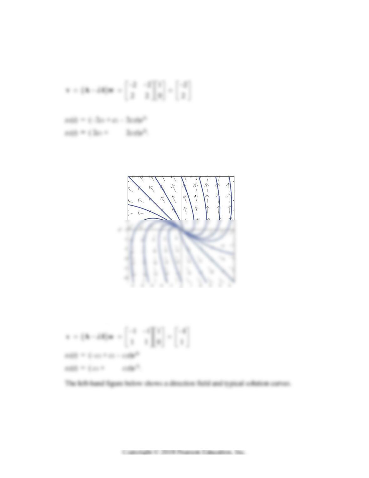
1. Characteristic equation
2 + 6
+ 9 = 0
Repeated eigenvalue
= –3
Generalized eigenvector w = [1 0]T
2. Characteristic equation
2 – 4
+ 4 = 0
Repeated eigenvalue
= 2
Generalized eigenvector w = [1 0]T
Section 7.6: Multiple Eigenvalue Solutions 447
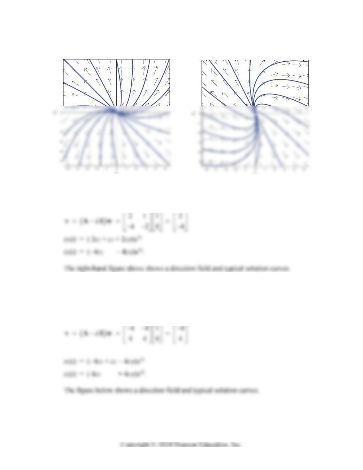
3. Characteristic equation
2 – 6
+ 9 = 0
Repeated eigenvalue
= 3
Generalized eigenvector w = [ 1 0]T
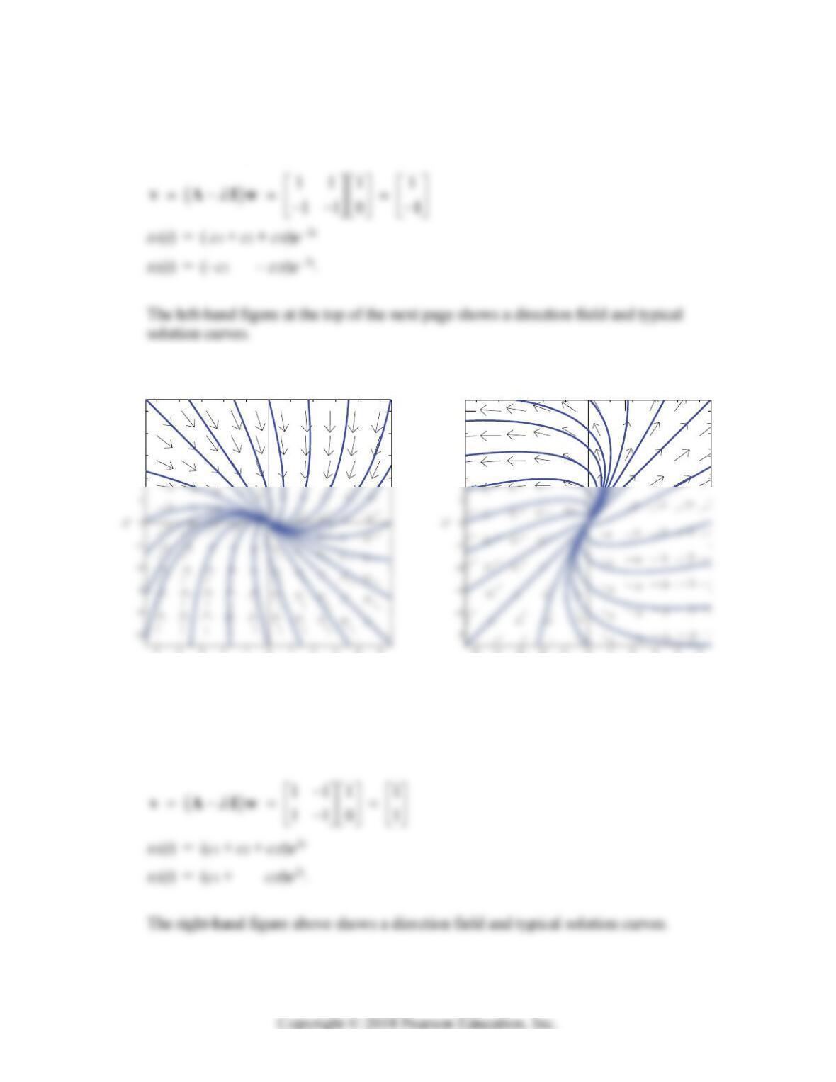
The figure at the top of the next page shows a direction field and typical solution curves.
2
3
4
5
x1
4. Characteristic equation
2 – 8
+ 16 = 0
Repeated eigenvalue
= 4
Generalized eigenvector w = [ 1 0]T
448 Chapter 7: Linear Systems of Differential Equations
1
2
3
4
5
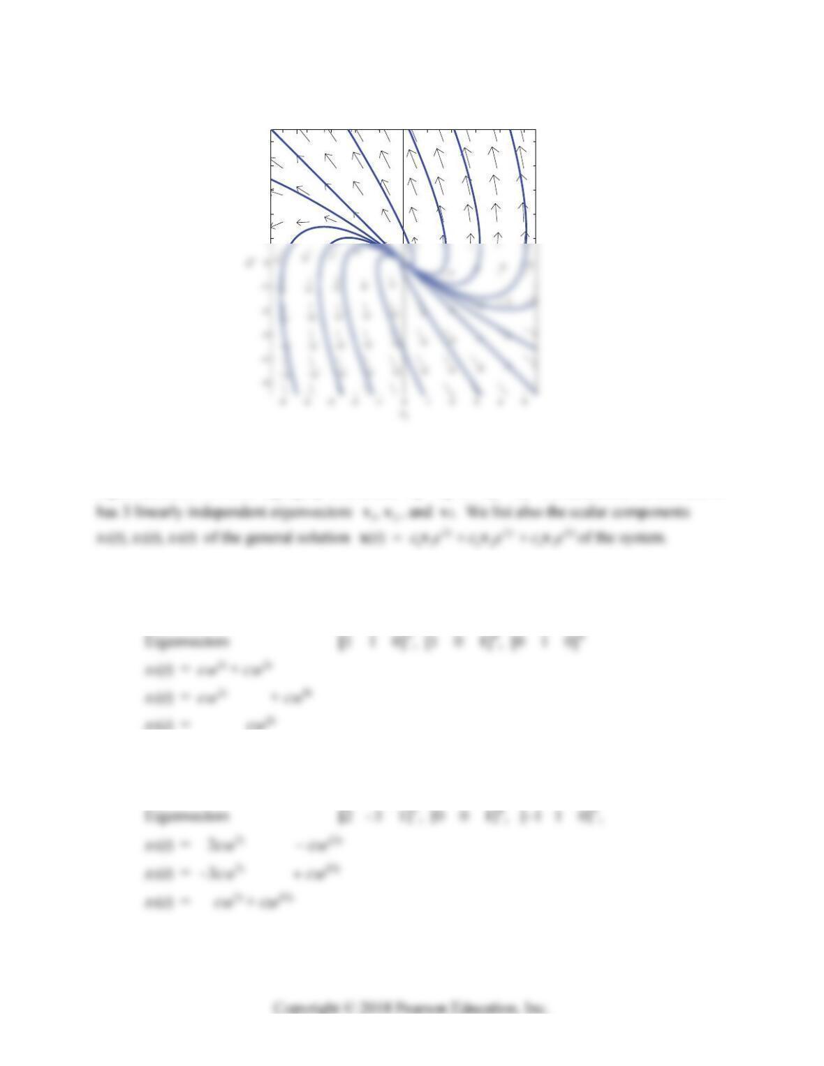
5. Characteristic equation
2 – 10
+ 25 = 0
Repeated eigenvalue
= 5
Generalized eigenvector w = [1 0]T
6. Characteristic equation
2 – 10
+ 25 = 0
Repeated eigenvalue
= 5
Generalized eigenvector w = [ 1 0]T
1
2
3
4
5
x1
Section 7.6: Multiple Eigenvalue Solutions 449
1
2
3
4
5
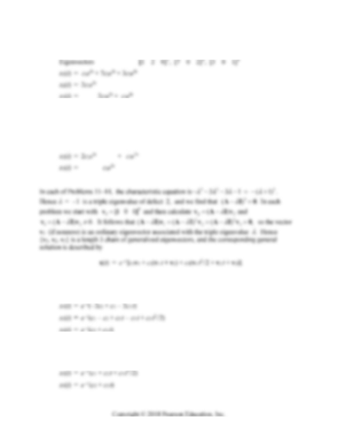
In each of Problems 7–10 the characteristic polynomial is easily calculated by expansion along
the row or column of A that contains two zeros. The matrix A has only two distinct
eigenvalues, so we write 123
,,
with either 12 23
or .
Nevertheless, we find that it
7. Characteristic equation 32 2
13 40 36 ( 2) ( 9)
Eigenvalues
= 2, 2, 9
8. Characteristic equation 32 2
33 351 1183 ( 13) ( 7)
Eigenvalues
= 7, 13, 13
450 Chapter 7: Linear Systems of Differential Equations
9. Characteristic equation 32 2
19 115 225 ( 5) ( 9)
Eigenvalues
= 5, 5, 9
10. Characteristic equation 32 2
13 51 63 ( 3) ( 7)
Eigenvalues
= 3, 3, 7
Eigenvectors [5 2 0]T, [–3 0 1]T, [2 1 0]T
x1(t) = 5c1e3t – 3c2e3t + 2c3e7t
We give the scalar components x1(t), x2(t), x3(t) of x(t).
11. v1 = [0 1 0]T, v2 = [–2 –1 1]T, v3 = [1 0 0]T
12. v1 = [1 1 0]T, v2 = [0 0 1]T, v3 = [1 0 0]T
x1(t) = e–t(c1 + c3 + c2 t + c3 t2/2)
Section 7.6: Multiple Eigenvalue Solutions 451
13. Here we are stymied initially, because if v3 = [1 0 0]T then 3
()
AIv0 does not
qualify as a (nonzero) generalized eigenvector. We there make a fresh start with
v3 = [0 1 0]T, and now we get the desired nonzero generalized eigenvectors upon
14. v1 = [5 –25 –5]T, v2 = [1 –5 4]T, v3 = [1 0 0]T
x1(t) = e–t(5c1 + c2 + c3 + 5c2 t + c3 t + 5c3 t2/2)
x2(t) = e–t(–25c1 – 5c2 – 25c2 t – 5c3 t – 25c3 t2/2)
x3(t) = e–t(–5c1 + 4c2 – 5c2 t + 4c3 t – 5c3 t2/2)
In each of Problems 15–18, the characteristic equation is 32 3
331 (1)
.
We give the scalar components x1(t), x2(t), x3(t) of x(t).
15. u1 = [3 –1 0]T u
2 = [0 0 1]T
v
1 = [–3 1 1]T v
2 = [1 0 0]T
452 Chapter 7: Linear Systems of Differential Equations
16. u1 = [3 –2 0]T u
2 = [3 0 –2]T
v
1 = [0 –2 2]T v
2 = [1 0 0]T
17. u1 = [2 0 –9]T u
2 = [1 –3 0]T
v
1 = [0 6 –9]T v
2 = [0 1 0]T
18. u1 = [–1 0 1]T u 2 = [–2 1 0]T
v
1 = [0 1 –2]T v2 = [1 0 0]T
19. Characteristic equation
4 – 2
2 + 1 = 0
Double eigenvalue
= –1 with eigenvectors
v1 = [1 0 0 1]T and v2 = [0 0 1 0]T.
Section 7.6: Multiple Eigenvalue Solutions 453
Scalar components
20. Characteristic equation 43 2
8243216
= (
– 2)4 = 0
Eigenvalue
= 2 with multiplicity 4 and defect 3.
We find that 3
()0
AI but 4
()0.
AI We therefore start with
v4 = [0 0 0 1]T and define 34
(),
vAIv23
(),
vAIv
23
(),
vAIvand
12
()0.
vAIv This gives the length 4 chain {v1, v2, v3, v4} with
with scalar components
21. Characteristic equation 432
4641
= (
– 1)4 = 0
Eigenvalue
= 1 with multiplicity 4 and defect 2.
We find that 2
()0
AI but 3
()0.
AI We therefore start with
v3 = [1 0 0 0]T and define 23
()
vAIvand 12
()0,
vAIv thereby
obtaining the length 3 chain {v1, v2, v3} with
454 Chapter 7: Linear Systems of Differential Equations
Then we find the second ordinary eigenvector v4 = [0 0 1 0]T. The corresponding
general solution
22. Same eigenvalue and chain structure as in Problem 21, but with generalized eigenvectors
v
1 = [1 0 0 –2]T v
2 = [3 –2 1 –6]T
v
3 = [0 1 0 0]T v
4 = [1 0 0 0]T
where {v1, v2, v3} is a length 3 chain and v4 is an ordinary eigenvector. The general
solution x(t) defined as in Problem 21 has scalar components
In Problems 23 and 24 there are only two distinct eigenvalues 12
and .
However, the
eigenvector equation ( ) 0
AIv yields the three linearly independent eigenvectors v1, v2,
and v3 that are given. We list the scalar components of the corresponding general solution
122
11 2 2 3 3
() .
ttt
tcecece
xvvv
23.
1 = –1: {v1} with v1 = [1 –1 2]T
2 = 3: {v2} with v2 = [4 0 9]T and
{v3} with v3 = [0 2 1]T