Section 7.6: Multiple Eigenvalue Solutions 455
24.
1 = –2: {v1} with v1 = [5 3 –3]T
2 = 3: {v2} with v2 = [4 0 –1]T and
{v3} with v3 = [2 –1 0]T
Scalar components
e
25. {v1, v2, v3} with
v
1 = [–1 0 –1]T, v
2 = [–4 –1 0]T, v
3 = [1 0 0]T
Scalar components
26. {v1, v2, v3} with
v
1 = [0 2 2]T, v
2 = [2 1 –3]T, v
3 = [1 0 0]T
General solution
27. We find that the triple eigenvalue
= 2 has the two linearly independent eigenvectors
[1 1 0]T and [–1 0 1]T. Next we find that ()0
AI but 2
()0.
AI We
therefore start with v2 = [1 0 0]T and define
456 Chapter 7: Linear Systems of Differential Equations
28. {v1, v2, v3} with
v
1 = [119 –289 0]T, v2 = [–17 34 17]T, v3 = [1 0 0]T
General solution
29.
= –1: {v1, v2} with v1 = [1 –3 –1 –2]T and v2 = [0 1 0 0]T,
= 2: {u1, u2} with u1 = [0 –1 1 0]T and u2 = [0 0 2 1]T
Scalar components
30.
= –1: {v1, v2} with v1 = [0 1 –1 –3]T and v2 = [0 0 1 2]T,
= 2: {u1, u2} with u1 = [–1 0 0 0]T and u2 = [0 0 3 5]T
Section 7.6: Multiple Eigenvalue Solutions 457
Scalar components
31. We have the single eigenvalue
= 1 of multiplicity 4. Starting with
v3 = [1 0 0 0]T, we calculate 23
()
vAIv and 12
(),
vAIv0
and find
that 1
().
AIv0 Therefore {v1, v2, v3} is a length 3 chain based on the ordinary
eigenvector v1. Next, the eigenvector equation ( )
AIv0 yields the second linearly
independent eigenvector v4 = [0 1 3 0]T. With
32. Here we find that the matrix A has five linearly independent eigenvectors:
= 2: eigenvectors v
1 = [8 0 –3 1 0]T and v2 = [1 0 0 0 3]T
= 3: eigenvectors v
3 = [3 –2 –1 0 0]T, v4 = [2 –2 0 –3 0]T,
v
5 = [1 –1 0 0 3]T
458 Chapter 7: Linear Systems of Differential Equations
33. The chain {v1, v2} was found using the matrices
4410 1 00
44 0 1 0010
0 0 4 4 0001
0044 0000
ii
i
i
i
AI
where signifies reduction to row-echelon form. The resulting real-valued solution
vectors are
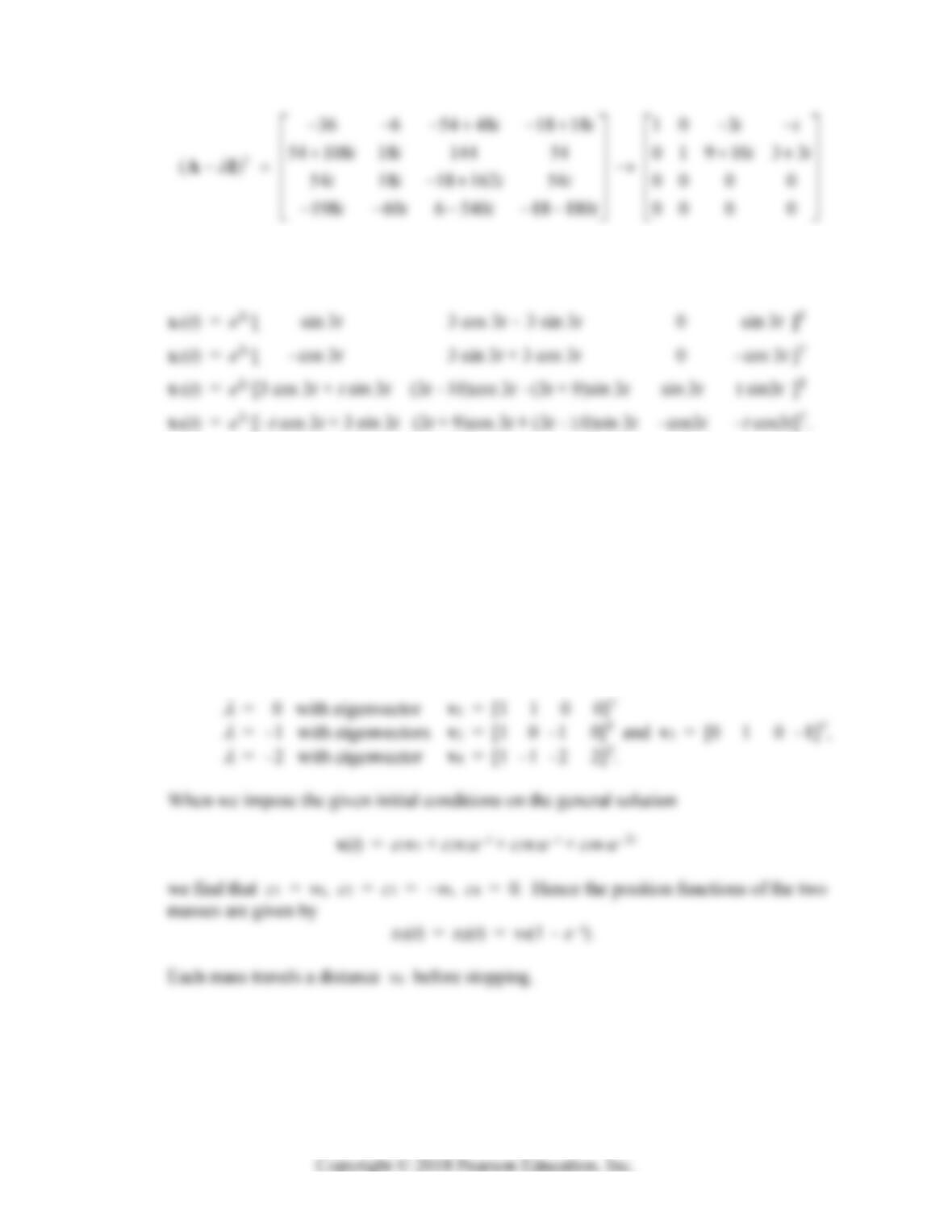
34. The chain {v1,v2} was found using the matrices
Section 7.6: Multiple Eigenvalue Solutions 459
where
signifies reduction to row-echelon form. The resulting real-valued solution
vectors are
35. The coefficient matrix
0010
0001
11 2 1
1112
A
has eigenvalues
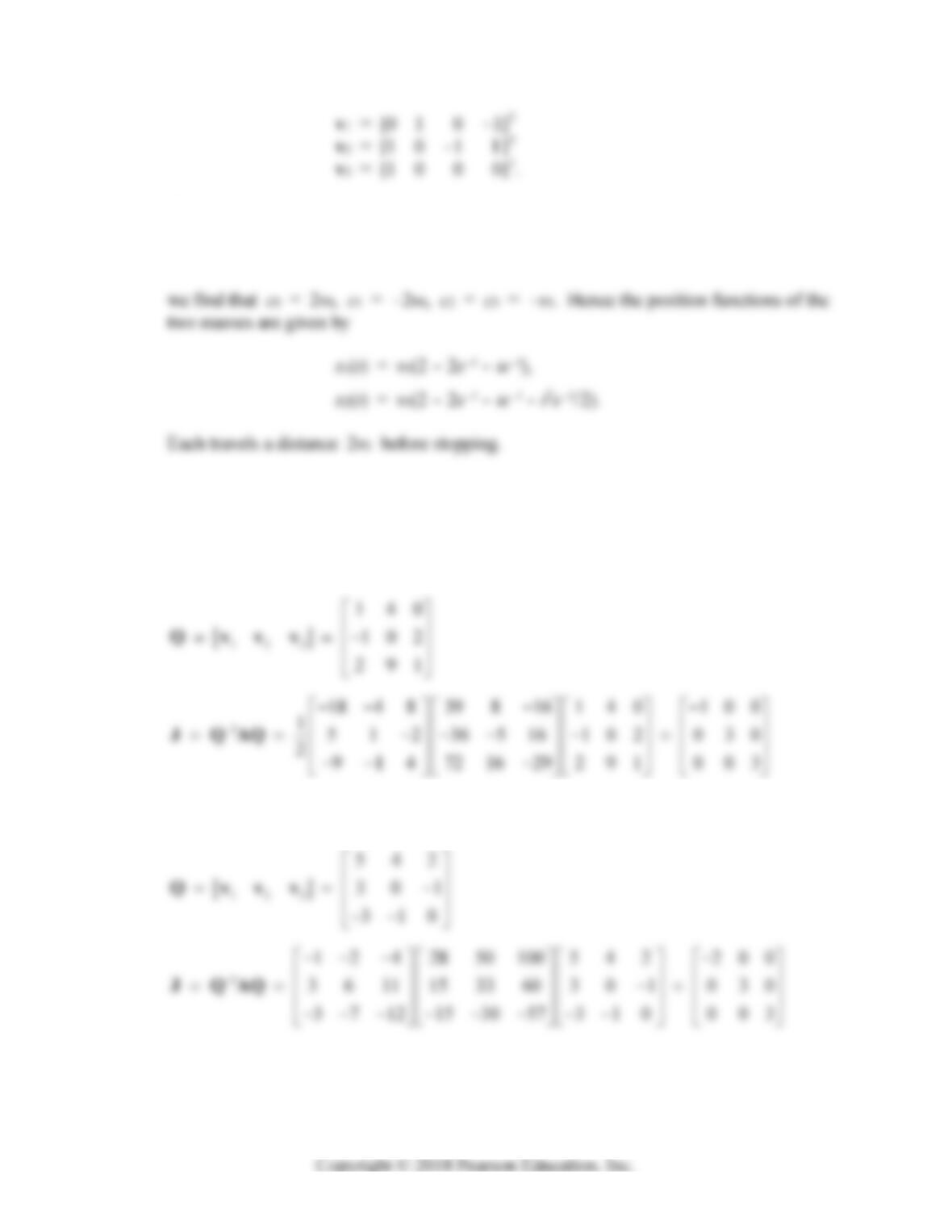
36. The coefficient matrix is the same as in Problem 35 except that a44 = –1. Now the
matrix A has the eigenvalue
= 0 with eigenvector v0 = [1 1 0 0]T, and the
triple eigenvalue
= –1 with associated length 2 chain {v1, v2, v3} consisting of the
generalized eigenvectors
460 Chapter 7: Linear Systems of Differential Equations
When we impose the given initial conditions on the general solution
x(t) = c0v0 + e–t [c1v1 + c2(v1t + v2) + c3(v1t2/2 + v2t + v3)]
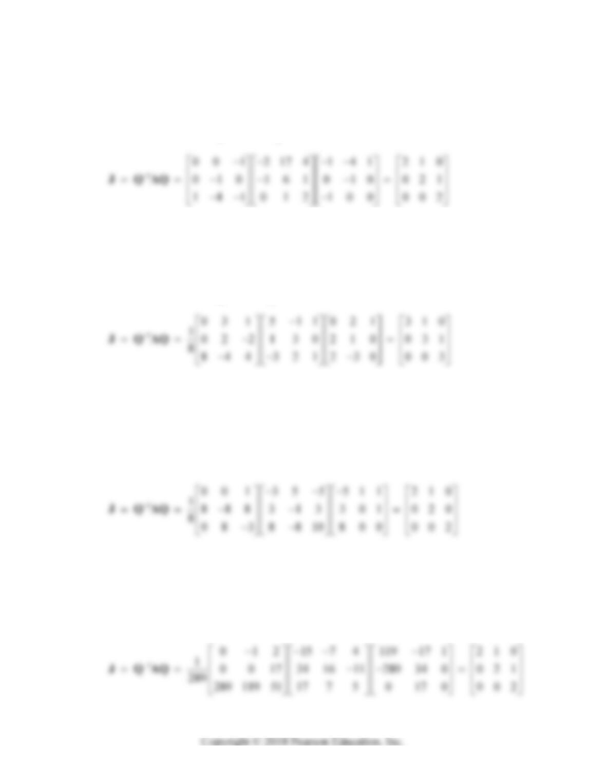
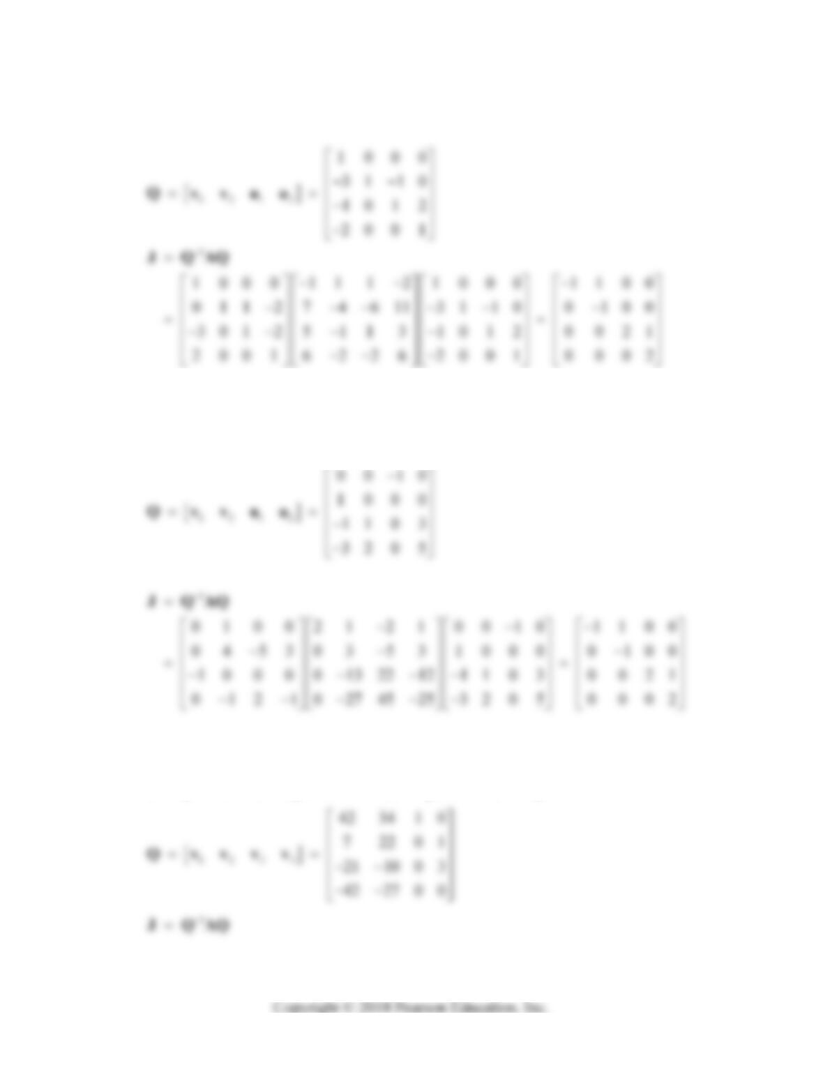
In Problems 37–46 we use the eigenvectors and generalized eigenvectors found in Problems 23–32
to construct a matrix Q such that J = Q–1AQ is a Jordan normal form of the given matrix A.
37. v1 = [1 –1 2]T, v2 = [4 0 9]T, v3 = [0 2 1]T
38. v1 = [5 3 –3]T, v2 = [4 0 –1]T, v3 = [2 –1 0]T
Section 7.6: Multiple Eigenvalue Solutions 461
39. v1 = [–1 0 –1]T, v2 = [–4 –1 0]T, v3 = [1 0 0]T
123
141
010
100
Qvvv
40. v1 = [0 2 2]T, v2 = [2 1 –3]T, v3 = [1 0 0]T
123
021
210
230
Qvvv
41. v1 = T
[5 3 8], v2 = [1 0 0]T, v3 = [1 1 0]T
123
511
301
800
Qvvv
42. v1 = [119 –289 0]T, v2 = [–17 34 17]T, v3 = [1 0 0]T
123
119 17 1
289 34 0
0170
Qvvv
462 Chapter 7: Linear Systems of Differential Equations
43. v1 = [1 –3 –1 –2]T, v2 = [0 1 0 0]T,
u
1 = [0 –1 1 0]T, u2 = [0 0 2 1]T
44. v1 = [0 1 –1 –3]T, v2 = [0 0 1 2]T,
u1 = [–1 0 0 0]T u2 = [0 0 3 5]T
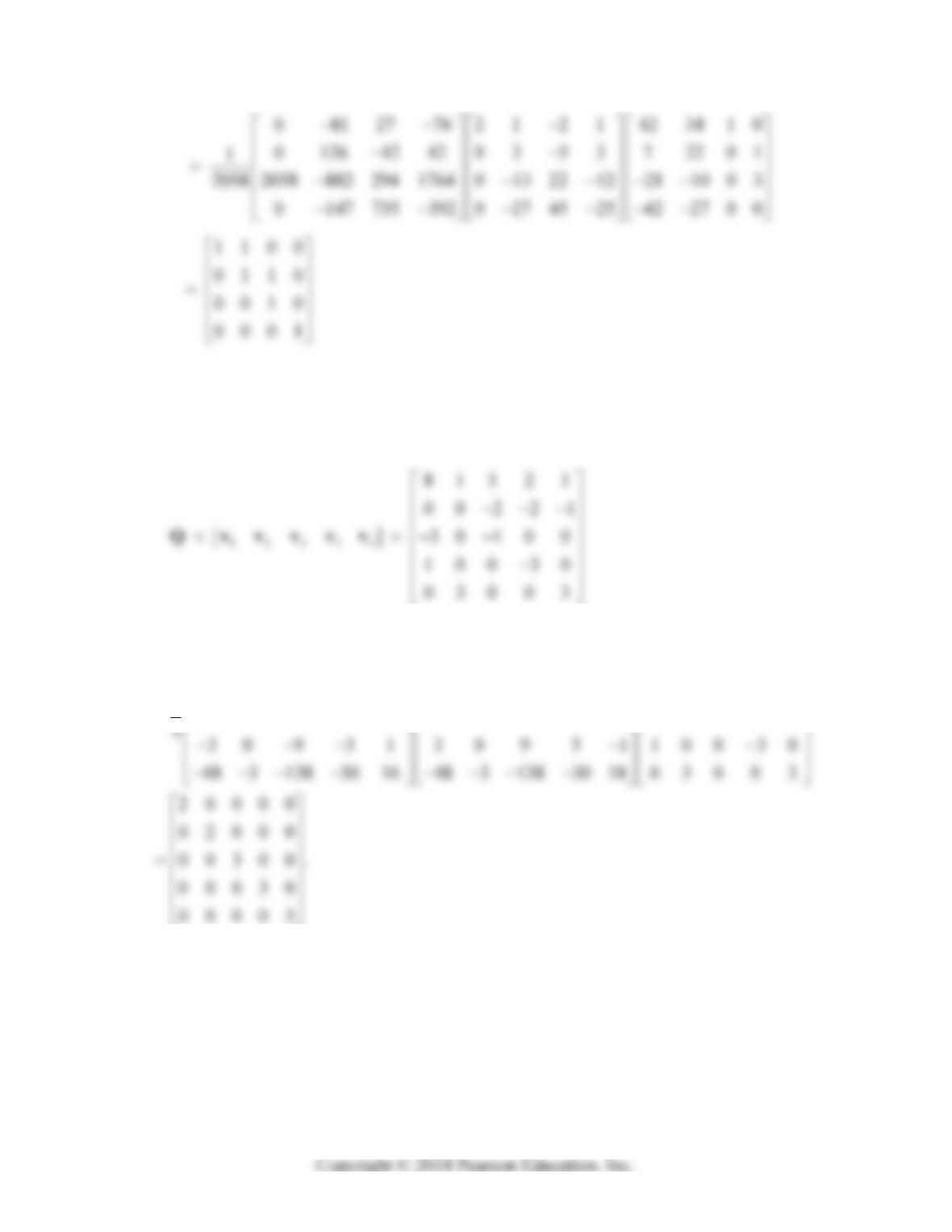
45. v1 = [42 7 –21 –42]T, v2 = [34 22 –10 –27]T,
v
3 = [1 0 0 0]T, v4 = [0 1 3 0]T
Section 7.6: Multiple Eigenvalue Solutions 463
46. v1 = [8 0 –3 1 0]T, v2 = [1 0 0 0 3]T
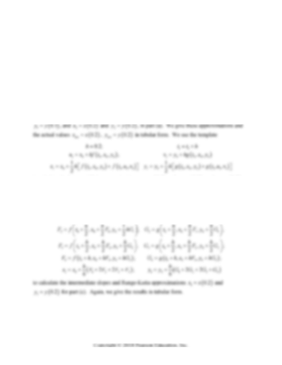
v3 = [3 –2 –1 0 0]T, v4 = [2 –2 0 –3 0]T, v5 = [1 –1 0 0 3]T
1
9 0 27 6 3 11 1 26 6 3 8 1 3 2 1
48 3 138 30 15 0 3 0 0 0 0 0 2 2 1
127 0 78 18 9 9 0 24 6 3 3 0 1 0 0
JQAQ
464 Chapter 7: Linear Systems of Differential Equations
SECTION 7.7
NUMERICAL METHODS FOR SYSTEMS
In Problems 1-8 we first write the given system in the form
,,
x
ftxy
,,ygtxy
. Then
we use the template
10
10 000 1 0 000
21 111 2 1 111
0.1;
,, ; ,,
,, ; ,,
h tth
x
xhftxy y yhgtxy
x
xhftxy y yhgtxy
(with the given values of 0
t, 0
x
, and 0
y
) to calculate the Euler approximations
10.1xx and
to calculate the improved Euler approximations
10.2ux and
10.2uy, and
10.2xx
and
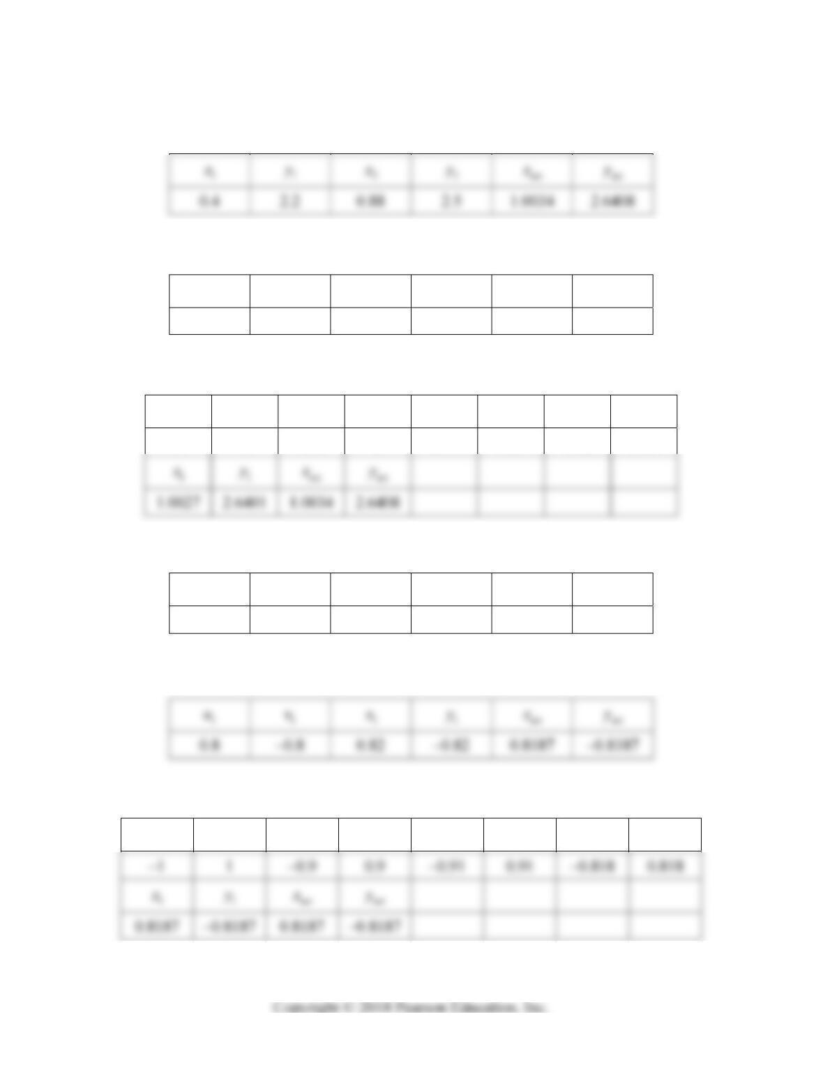
10.2yy, in part (b). We give these approximations and the actual values
act 0.2xx,
act 0.2yy in tabular form. We use the template
1 000 1 000
0.2;
,, ; ,, ;
h
Fftxy Ggtxy
Section 7.7: Numerical Methods for Systems 465
1. (a)
x
y
x
y
x
y
(b)
1
u 1
v 1
x
1
y
act
x
act
y
0.8 2.4 0.96 2.6 1.0034 2.6408
(c)
1
F 1
G 2
F
2
G 3
F 3
G 4
F
4
G
4 2 4.8 3 5.08 3.26 6.32 4.684
x
y
x
y
2. (a)
1
x
1
y
2
x
2
y
act
x
act
y
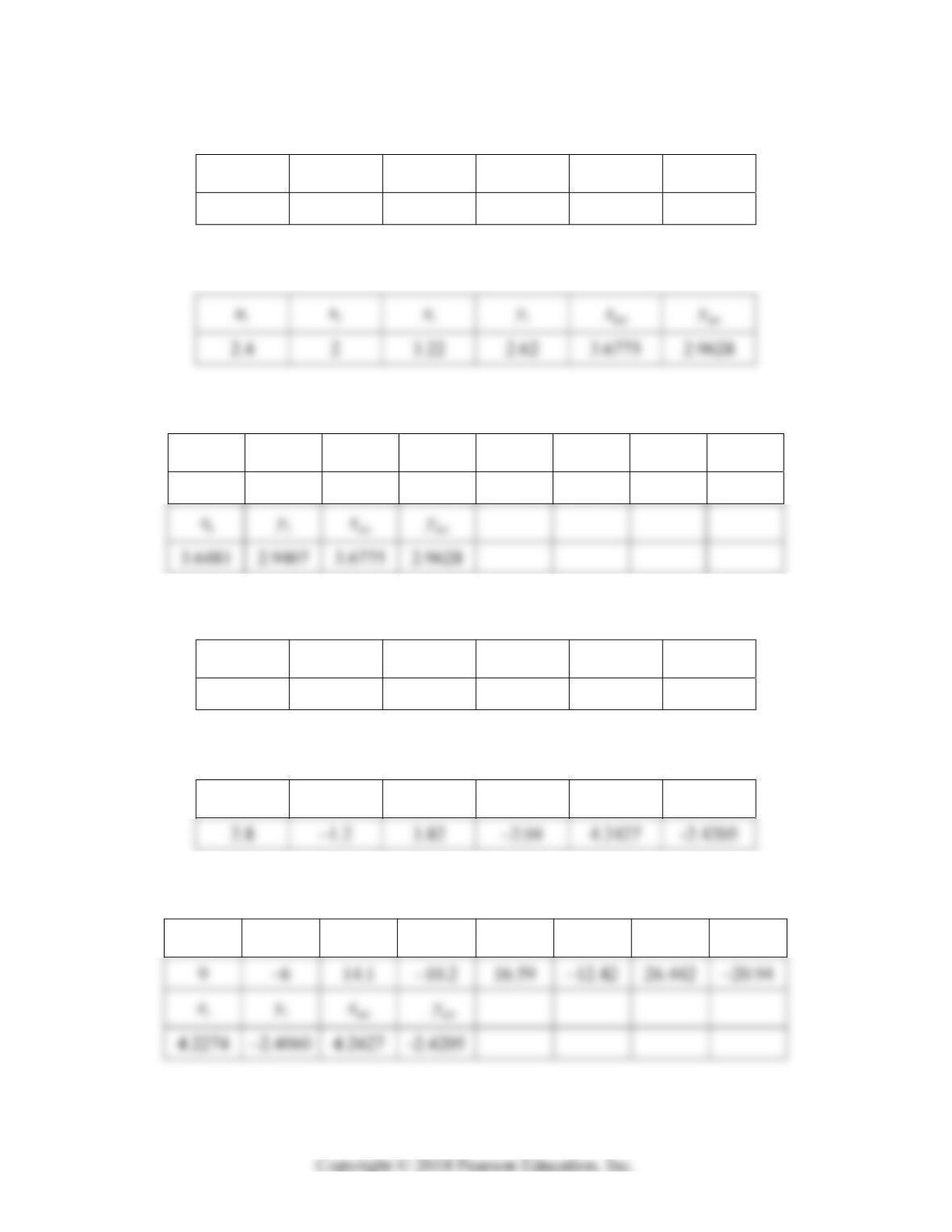
0.9 –0.9 0.81 –0.81 0.8187 –0.8187
(b)
x
y
x
y
(c)
1
F 1
G 2
F 2
G 3
F 3
G 4
F 4
G
x
y
x
y
466 Chapter 7: Linear Systems of Differential Equations
3. (a)
1
x
1
y
2
x
2
y
act
x
act
y
1.7 1.5 2.81 2.31 3.6775 2.9628
(b)
x
y
x
y
(c)
1
F 1
G 2
F
2
G 3
F 3
G 4
F
4
G
7 5 11.1 8.1 13.57 9.95 23.102 17.122
x
y
x
y
4. (a)
1
x
1
y
2
x
2
y
act
x
act
y
1.9 –0.6 3.31 –1.62 4.2427 -2.4205
(b)
1
u .. 1
x
1
y
act
x
act
y
(c)
1
F 1
G 2
F
2
G 3
F 3
G 4
F 4
G
x
y
x
y

Section 7.7: Numerical Methods for Systems 467
5. (a)
1
x
1
y
2
x
2
y
act
x
act
y
0.9 3.2 –0.52 2.92 -0.5793 2.4488
(b)
x
y
x
y
(c)
1
F 1
G 2
F
2
G 3
F 3
G 4
F 4
G
–11 2 –14.2 –2.8 –12.44 –3.12 –12.856 –6.704
x
y
x
y
6. (a)
1
x
1
y
2
x
2
y
act
x
act
y
–0.8 4.4 –1.76 4.68 -1.9025 4.4999
(b)
x
y
x
y
(c)
1
F 1
G 2
F
2
G 3
F 3
G 4
F 4
G
–8 4 –9.6 2.8 –9.52 2.36 –10.848 0.664
x
y
x
y
468 Chapter 7: Linear Systems of Differential Equations
7. (a)
x
y
x
y
x
y
(b)
1
u 1
v 1
x
1
y
act
x
act
y
3 1.6 3.24 1.76 3.2820 1.7902
(c)
1
F 1
G 2
F
2
G 3
F 3
G 4
F 4
G
x
y
x
y
8. (a)
1
x
1
y
2
x
2
y
act
x
act
y
0.9 –0.9 2.16 –0.63 2.5270 -0.3889
(b)
1
u 1
v 1
x
1
y
act
x
act
y
(c)
1
F 1
G 2
F
2
G 3
F 3
G 4
F 4
G
9 1 12.6 2.7 12.87 3.25 16.02 5.498
x
y
x
y
Section 7.7: Numerical Methods for Systems 469
In Problems 9-11 we use the same Runge-Kutta template as in part (c) of Problems 1–8 above,
and give both the Runge-Kutta approximate values with step sizes 0.1h and 0.05h, and
also the actual values.
9.
With 0.1h:
3.9 11 926x
6.2 01 177y
10.
With 0.1h:
1 1.31498x
y 1 1.02537
11.
With 0.1h:
1 0.05832x
1 0.56664y
12. We first convert the given initial value problem to the two-dimensional problem
13. With yx
we want to solve numerically the initial value problem
470 Chapter 7: Linear Systems of Differential Equations
When we run Program RK2DIM with step size 0.1h we find that the change of sign in
the velocity v occurs as follows:
t x v
14. Now we want to solve numerically the initial value problem
,00,
xy x
15. With
y
x
and with x in miles and in seconds, we want to solve numerically the initial
value problem
16. We first defined the MATLAB function
function xp = fnball(t,x)
% Defines the baseball system
% x1 = x = x3, x3 = -cvx
% x2 = y = x4, x4 = -cvy– g
Section 7.7: Numerical Methods for Systems 471
Then, using the n-dimensional program rkn with step size 0.1 and initial data
corresponding to the indicated initial inclination angles, we got the following results:
Angle Time Range
40 5.0 352.9
17. The data in Problem 16 indicate that the range increases when the initial angle is
decreased below 45. The further data
Angle Range
41.0 352.1
40.5 352.6
18. We “shoot” for the proper inclination angle by running program rkn (with 0.1h) as
follows:
Angle Range
60 287.1
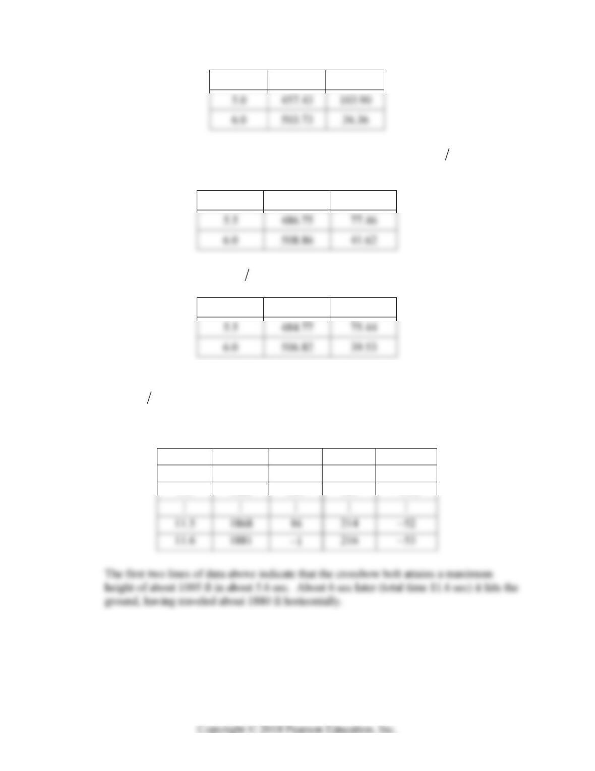
19. First we run program rkn (with 0.1h) with 0250 ft secv and obtain the following
results:
472 Chapter 7: Linear Systems of Differential Equations
t x y
Interpolation gives 494.4x when 50y. Then a run with 0255 ft secv gives the
following results:
t x y
Finally, a run with 0253 ft secv gives these results:
t x y
Now 500ftx when 50fty. Thus Babe Ruth’s home run ball had an initial velocity
of 253 ft sec .
20. A run of program rkn with 0.1h and with the given data yields the following results:
t x y v
5.5 989 539 162 0.95
5.6 1005 539 161 0.18
21. A run with 0.1h indicates that the projectile has a range of about 21,400ft 4.05mi
and a flight time of about 46 sec. It attains a maximum height of about 8970 ft in about
17.5 sec. At time 23sect it has its minimum velocity of about 368 ft/sec. It hits the
ground ( 23sect) at an angle of about 77 with a velocity of about 518 ft/sec.
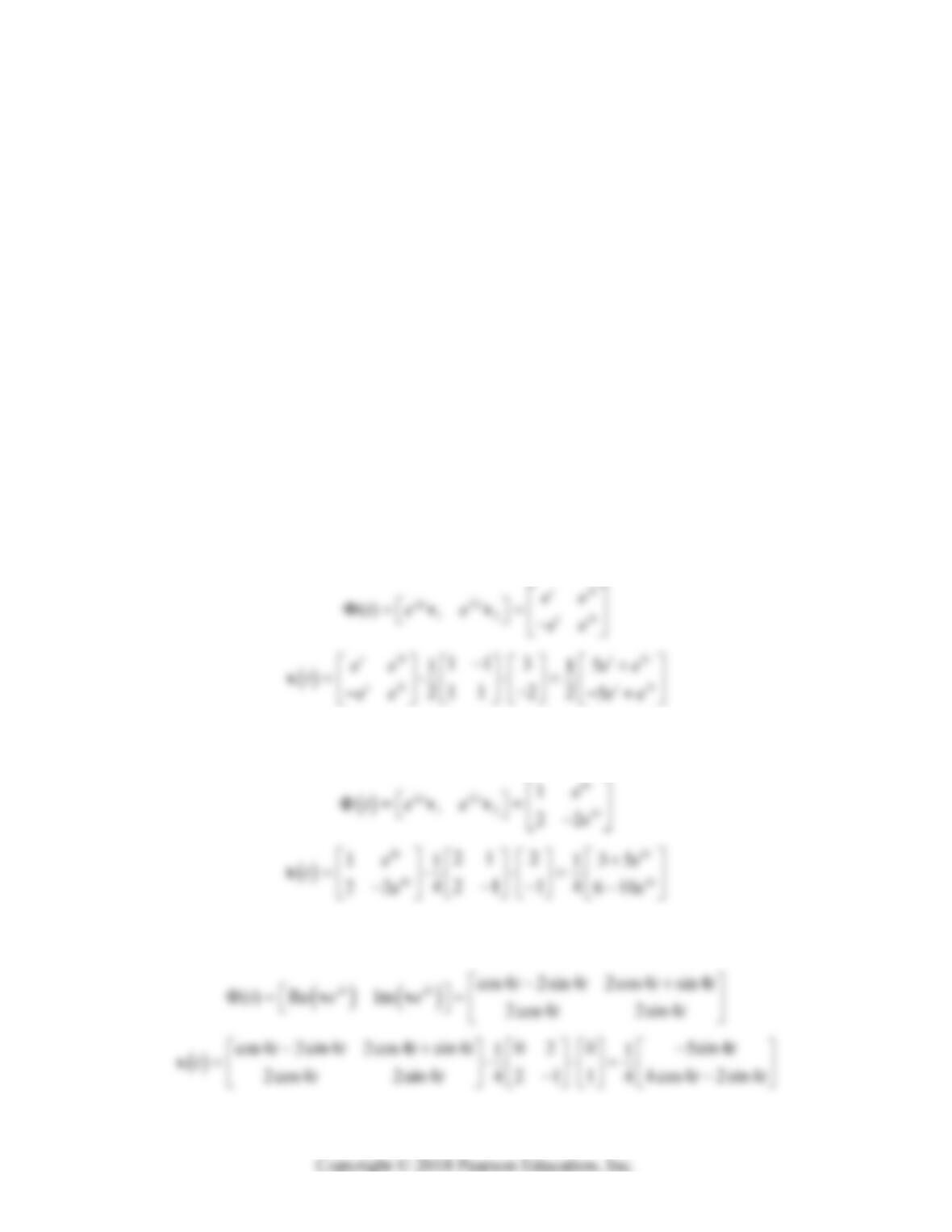
473
CHAPTER 8
MATRIX EXPONENTIAL METHODS
SECTION 8.1
MATRIX EXPONENTIALS AND LINEAR SYSTEMS
In Problems 1–8 we first use the eigenvalues and eigenvectors of the coefficient matrix A to find
first a fundamental matrix
t for the homogeneous system xAx
. Then we apply the
formula
1
0
0tt
xx to find the solution vector
tx that satisfies the initial condition
0
0xx. Formulas (11) and (12) in the text provide inverses of 22 and 33 matrices.
1. Eigensystem: 11
,
T
111v; 23
,
T
111v
2. Eigensystem: 10
,
T
112v; 24
, 24
,
T
212v
3. Eigensystem: 4i
,
T
12 2iv;
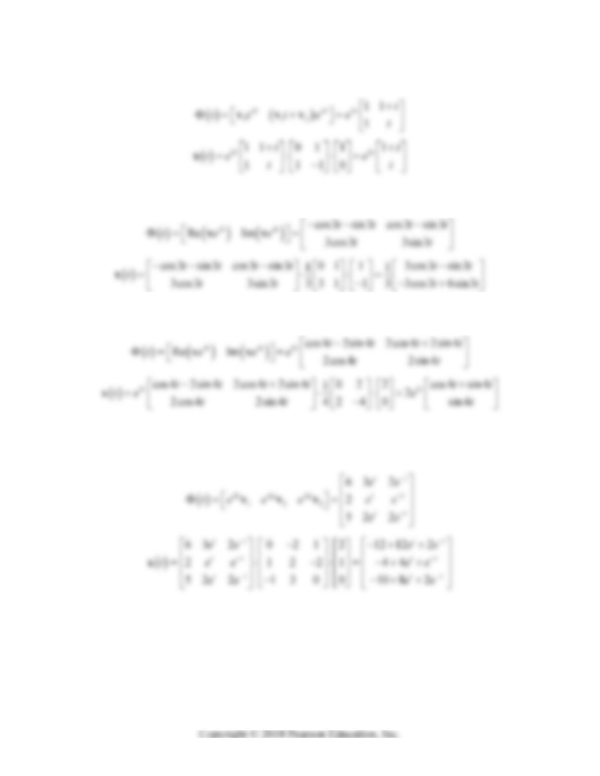
474 Chapter 8: Matrix Exponential Methods
4. Eigensystem: 2,2
, 12
{, }vv with
T
111v,
T
210v;
5. Eigensystem: 3i
,
T
13iv;
6. Eigensystem: 54i
,
T
12 2iv;
7. Eigensystem:
TT T
11 22 3 3
0, 6 2 5 ; 1, 3 1 2 ; 1, 2 1 2
vv v;
8. Eigensystem:
TTT
11 22 33
2, 011; 1, 110; 3, 111
vv v;