Section 8.1: Matrix Exponentials and Linear Systems 475
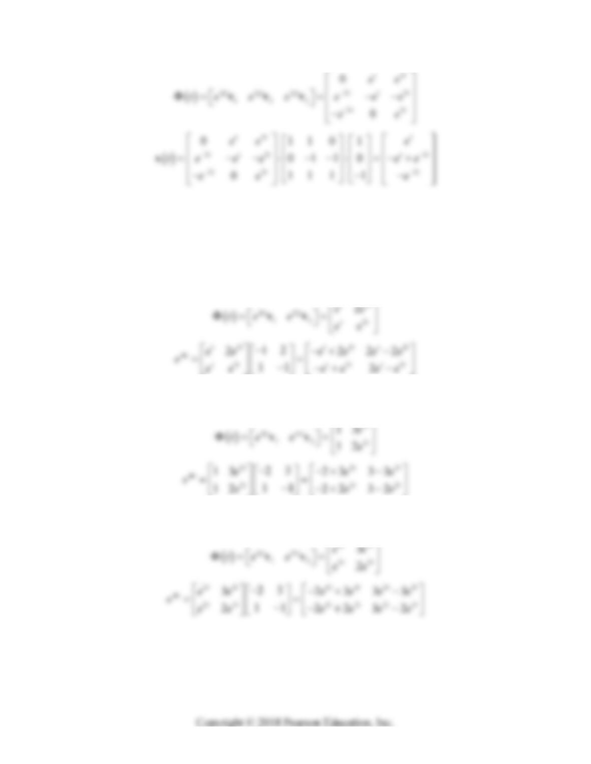
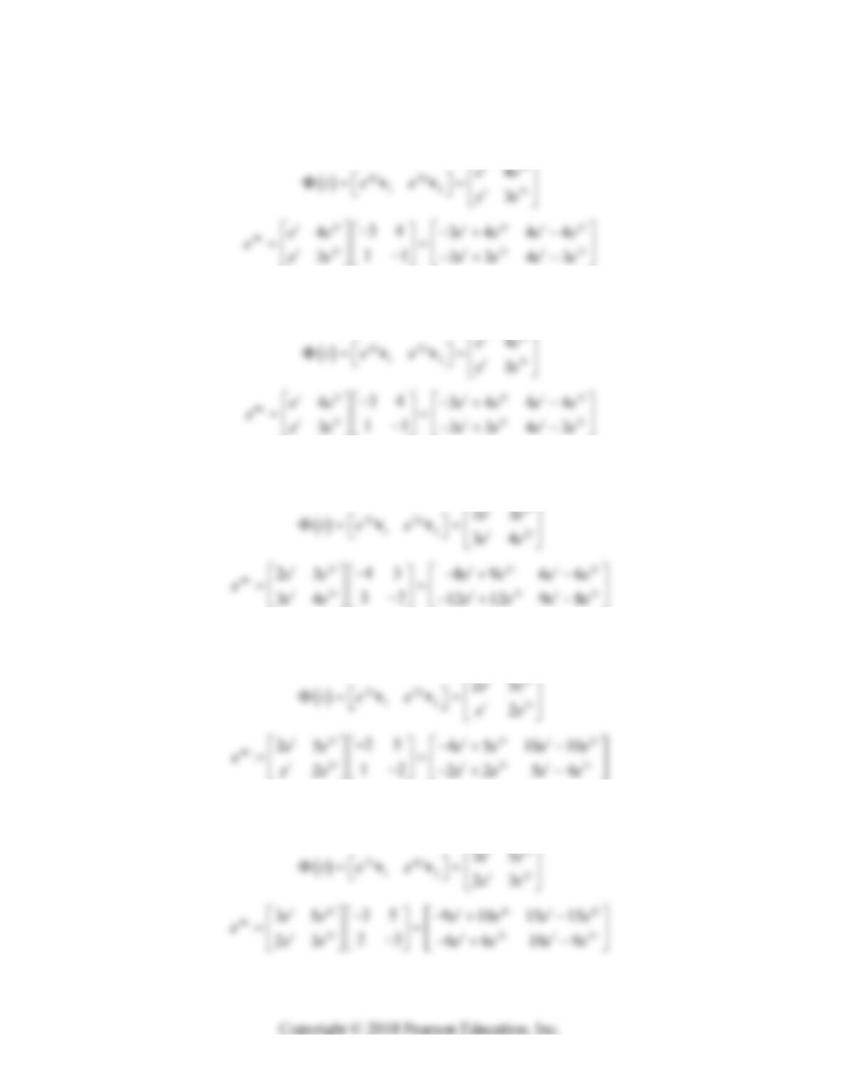
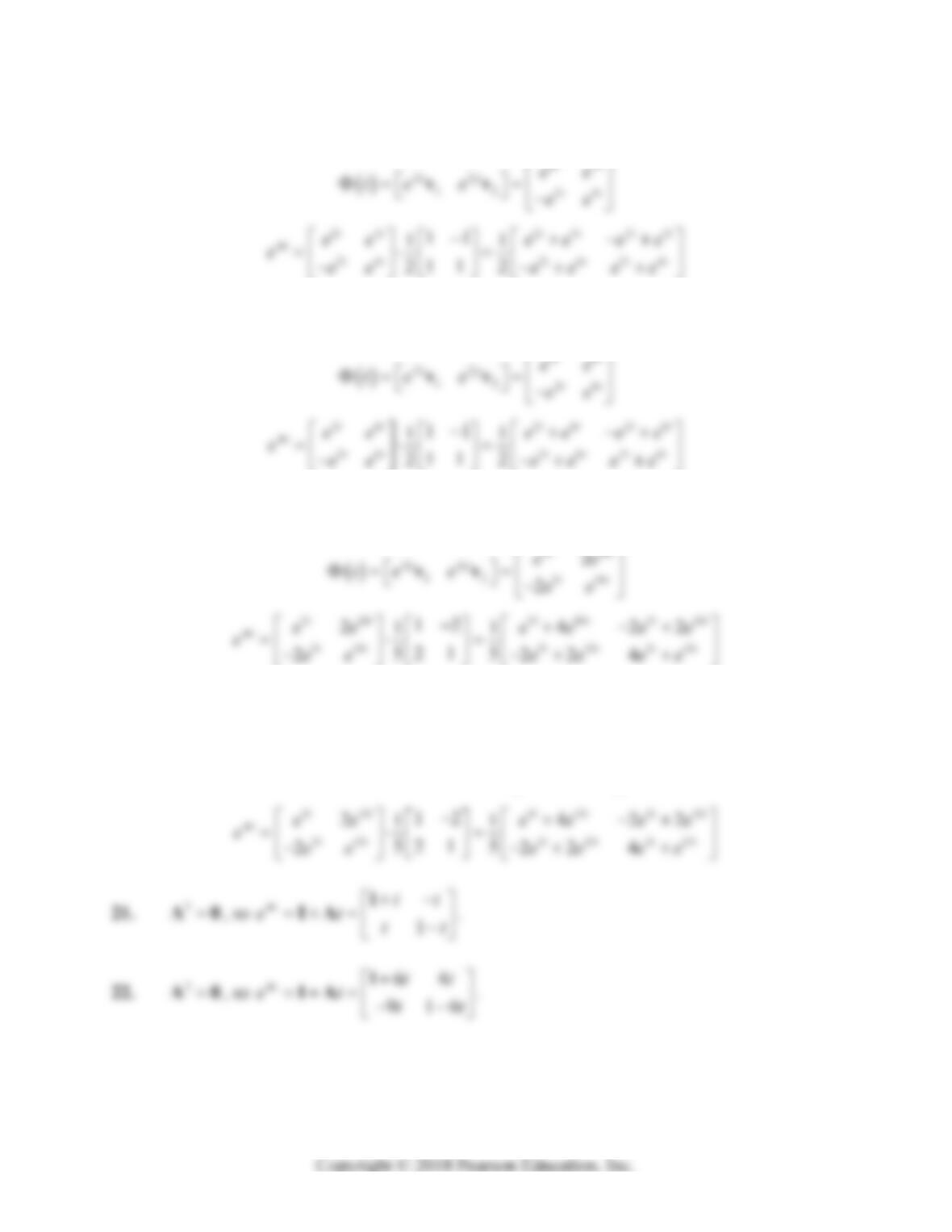
In each of Problems 9–20 we first solve the given linear system to find two linearly independent
solutions 1
x and 2
x, then set up the fundamental matrix
12
ttt
xx
, and finally
calculate the matrix exponential
1
0
t
et
A.
9. Eigensystem:
TT
11 2 2
1, 1 1 ; 3, 2 1
vv;
10. Eigensystem:
TT
11 2 2
0, 1 1 ; 2, 3 2
vv;
11. Eigensystem:
TT
11 22
2, 1 1 ; 3, 3 2
vv;
476 Chapter 8: Matrix Exponential Methods
12. Eigensystem:
TT
11 2 2
1, 1 1 ; 2, 4 3
vv;
13. Eigensystem:
TT
11 2 2
1, 1 1 ; 3, 4 3
vv
14. Eigensystem:
TT
11 2 2
1, 2 3 ; 3, 3 4
vv;
15. Eigensystem:
TT
11 2 2
1, 2 1 ; 2, 5 2
vv;
16. Eigensystem:
TT
11 2 2
1, 3 2 ; 2, 5 3
vv;
Section 8.1: Matrix Exponentials and Linear Systems 477
17. Eigensystem:
TT
11 2 2
2, 1 1 ; 4, 1 1
vv;
18. Eigensystem:
TT
11 22
2, 1 1 ; 6, 1 1
vv;
19. Eigensystem:
TT
11 2 2
5, 1 2 ; 10, 2 1
vv;
20. Eigensystem:
TT
11 2 2
5, 1 2 ; 15, 2 1
vv;
12
515
12 515
2
2
tt
tt
tt
ee
te e ee
vv
478 Chapter 8: Matrix Exponential Methods
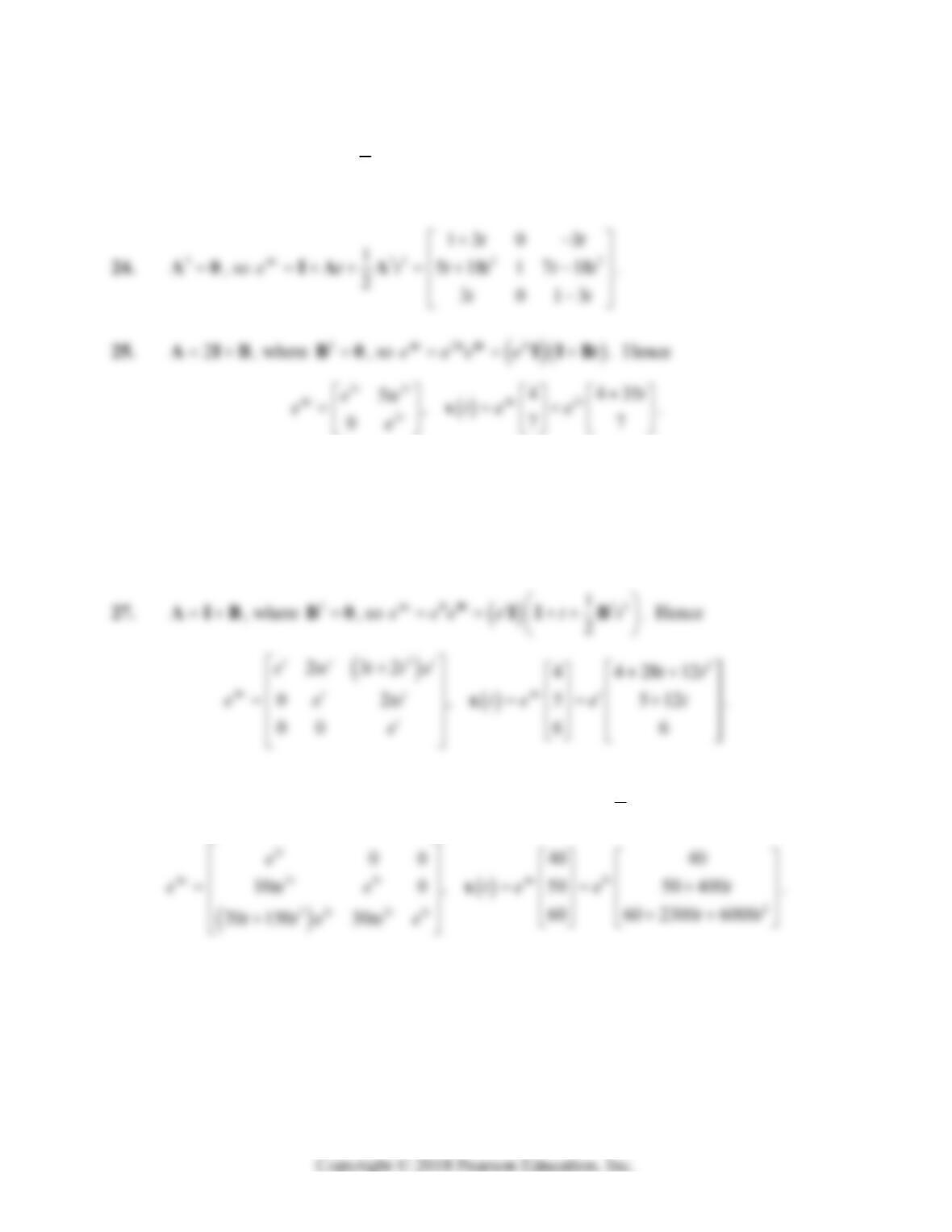
23. 3A0
, so
2
22 2
1
11
200 1
t
tttt
etttttt
AIA A .
26. 7AIB, where 2B0
, so
77ttt t
eee e t
AIB IIB. Hence
7
7
77
55
0,10 10 55
11
t
ttt
tt
e
etee
t
te e
AA
x.
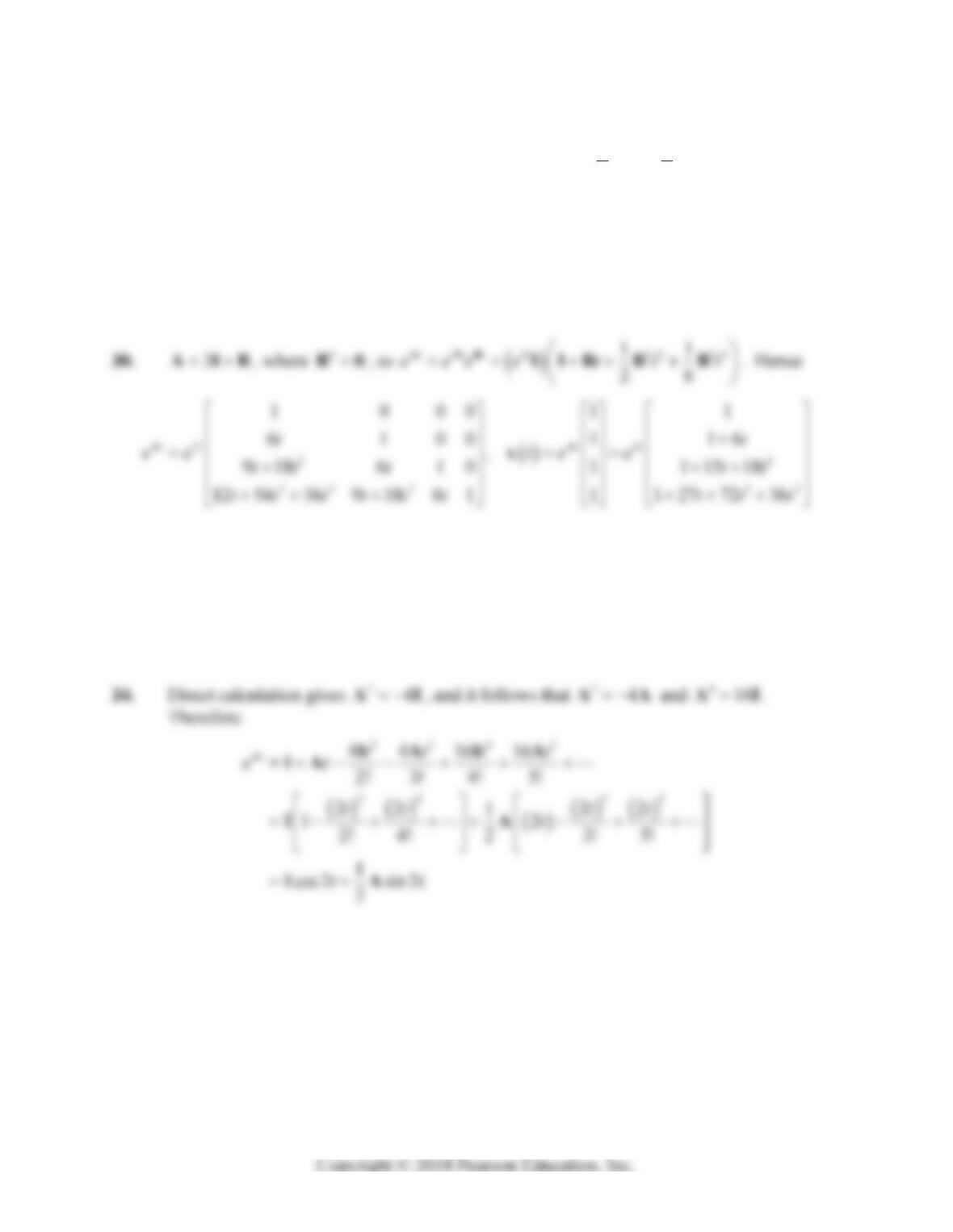
28. 5AIB, where 3B0, so
55 22
1
2
ttt t
eee e t t
AIB IIB B . Hence
Section 8.1: Matrix Exponentials and Linear Systems 479
29. AIB, where 4B0
, so
22 33
11
26
ttt t
eee e t t t
AIB IIB B B . Hence
223 23
22
1
12 3 6 4 6 4 19 12 4
1
01 6 36 19 6
,1
00 1 2 12
1
00 0 1 1
tt t t
tttttt ttt
ttt tt
ee te e
tt
A A
x.
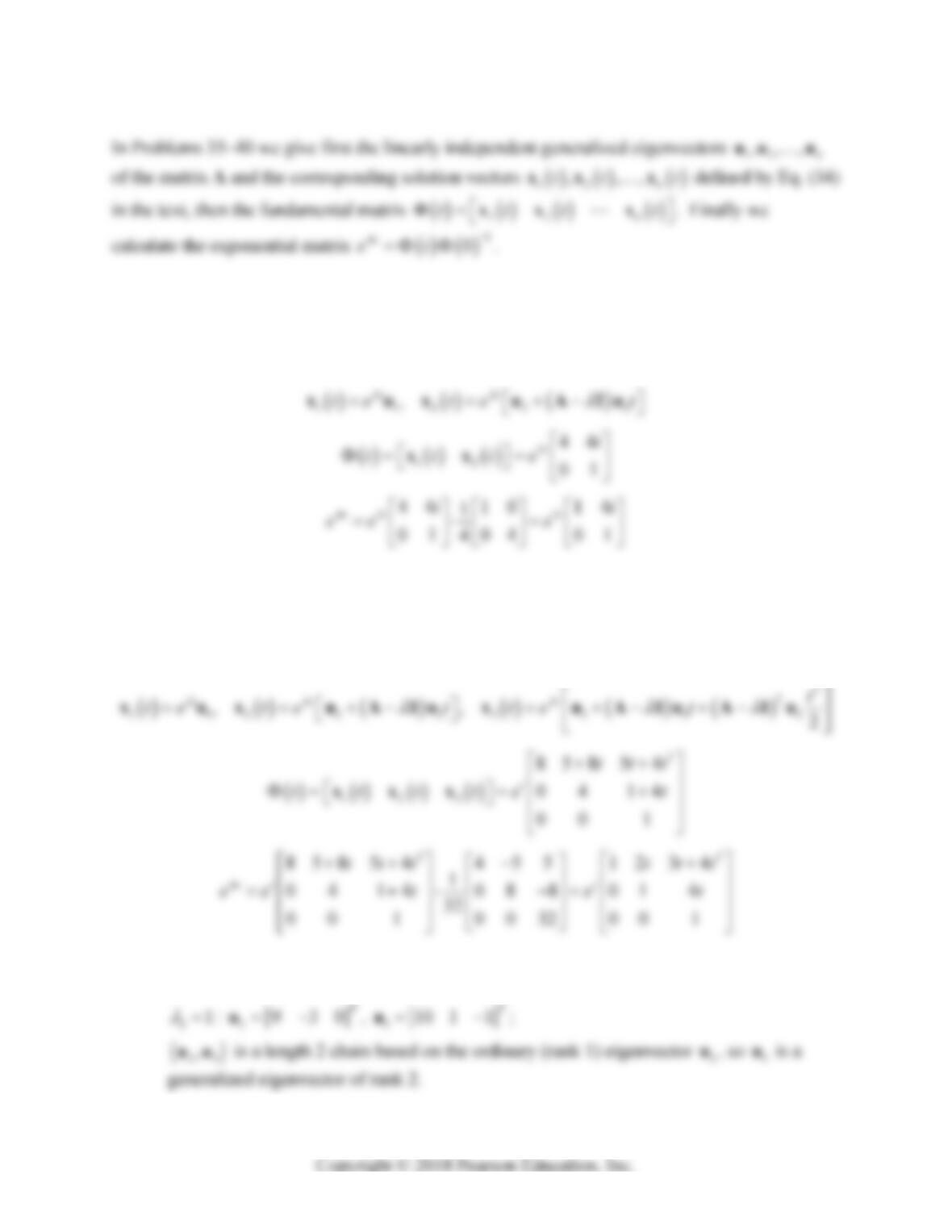
33. cosh sinh
cosh sinh sinh cosh
ttt
ett
tt
AIA , so the general solution of xAx
is
12
12
cosh sinh
sinh cosh
tctct
te ctc t
A
xc .
480 Chapter 8: Matrix Exponential Methods
35. 3
:
T
140u,
T
201u;
12
,uu is a length 2 chain based on the ordinary (rank 1) eigenvector 1
u, so 2
u is a
generalized eigenvector of rank 2.
36. 1
:
T
1800u,
T
2540u,
T
3011u;
123
,,uuu is a length 3 chain based on the ordinary (rank 1) eigenvector 1
u, so 2
u and
3
u are generalized eigenvectors of ranks 2 and 3 (respectively).
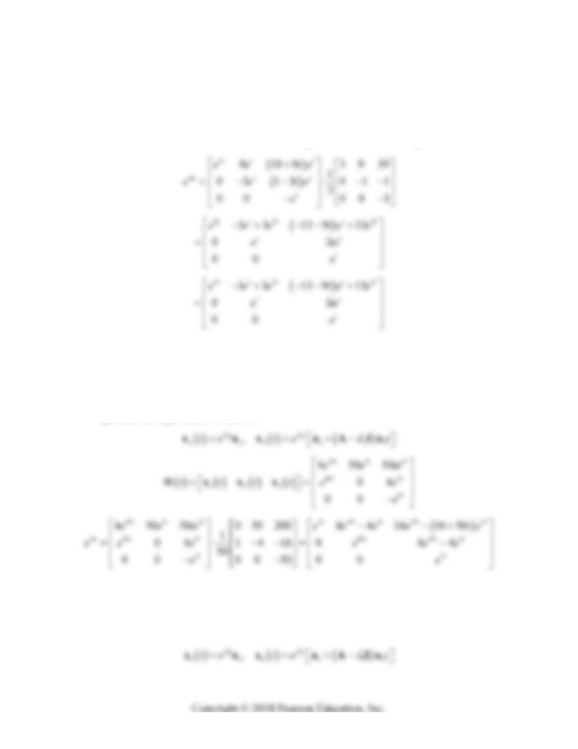
37. 12
:
T
1100u,
1
11
t
te
xu;
Section 8.1: Matrix Exponentials and Linear Systems 481
22
223 323
,
tt
te te t
xux uAIu
2
123
9109
03 13
00
tt t
tt
t
ee te
tttt e te
e
xxx
38. 110
:
T
1410u,
1
11
t
te
xu;
25
:
T
25000u,
T
304 1u;
23
,uu is a length 2 chain based on the ordinary (rank 1) eigenvector 2
u, so 3
u is a
generalized eigenvector of rank 2.
39. 21
:
T
13000u,
T
20100u;
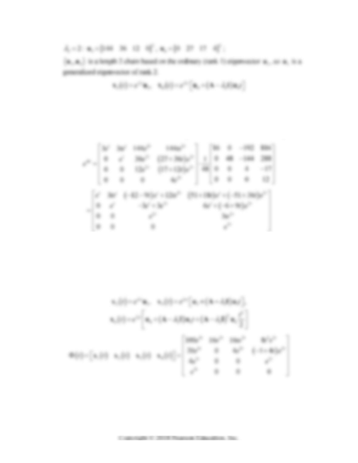
12
,uu is a length 2 chain based on the ordinary (rank 1) eigenvector 1
u, so 2
u is a
generalized eigenvector of rank 2.
482 Chapter 8: Matrix Exponential Methods
22
22
1234 22
2
3 3 144 144
0362736
0 0 12 17 12
00 0 4
tt t t
tt t
tt
t
ete e te
ee te
ttttt ete
e
xxxx
40. 13
:
T
1100 20 4 1u,
1
11
t
te
xu
;
2
:
T
216000u,
T
30400u,
T
40110u;
234
,,uuu is a length 3 chain based on the ordinary (rank 1) eigenvector 2
u, so 3
u and
4
u are generalized eigenvectors of ranks 2 and 3 (respectively).
Section 8.2: Nonhomogeneous Linear Systems 483
00 0
e
SECTION 8.2
NONHOMOGENEOUS LINEAR SYSTEMS
1. Substitution of the trial solution
p
x
ta,
p
yt b yields the equations
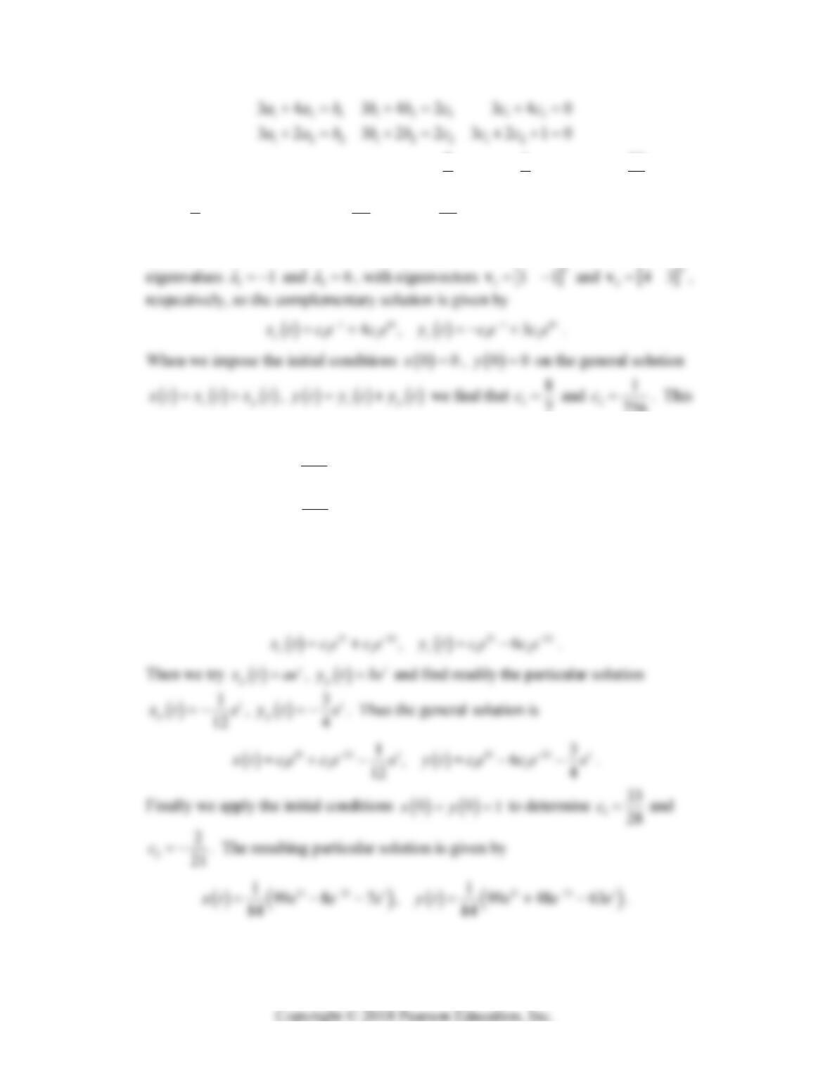
2. When we substitute the trial solution
11p
x
tabt ,
22p
yt a bt and collect
coefficients, we get the equations
3. When we substitute the trial solution
22
11 1 2 2 2
,
pp
x
a btct y a btct
and collect coefficients, we get the equations
484 Chapter 8: Matrix Exponential Methods
Working backwards, we solve first for 1
2
3
c and 2
1
2
c, then for 1
10
9
b and
2
7
6
b , and finally for 1
31
27
a and 2
41
36
a. This determines the particular solution
p
x
t,
p
yt
. Next, the coefficient matrix of the associated homogeneous system has
x
x
7
756
finally gives the desired particular solution
62
62
1864 4 868 840 504 ,
756
1864 3 861 882 378 .
756
tt
tt
xt e e t t
y
teett
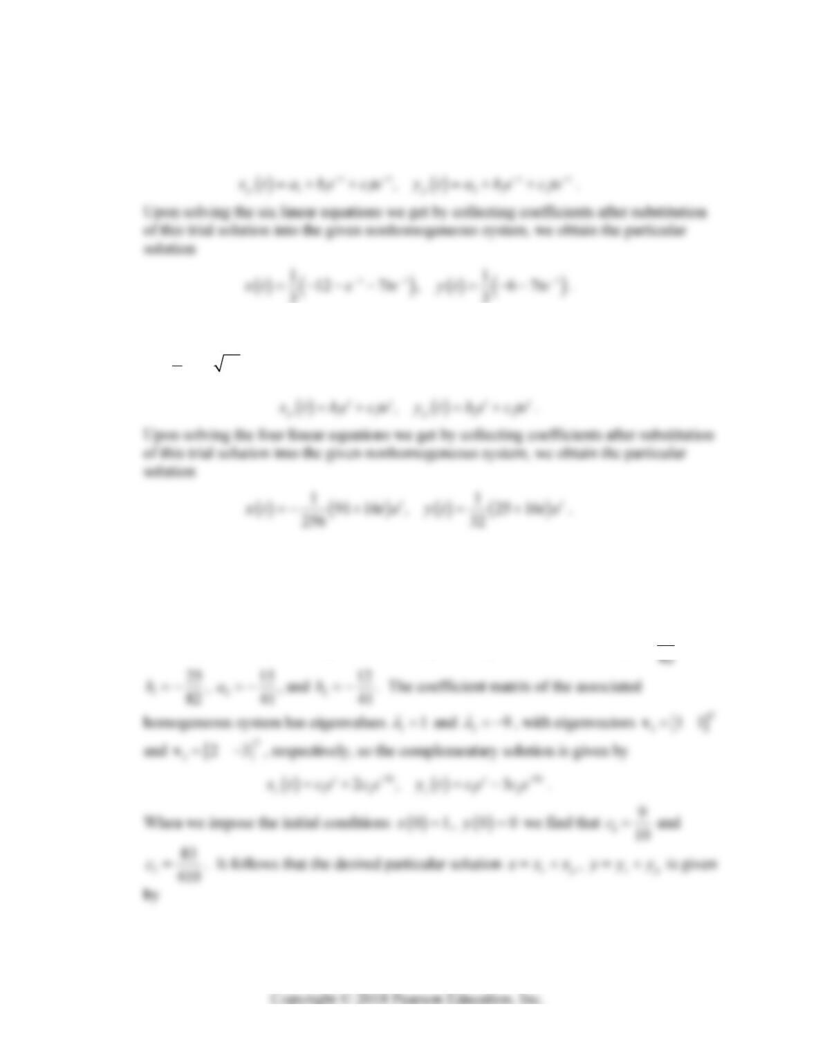
4. The coefficient matrix of the associated homogeneous system has eigenvalues 15
and 22
, with eigenvectors
T
111v and
T
216v, respectively, so the
complementary solution is given by
x
x
Section 8.2: Nonhomogeneous Linear Systems 485
5. The coefficient matrix of the associated homogeneous system has eigenvalues 11
and 25
, so the nonhomogeneous term t
e duplicates part of the complementary
solution. We therefore try the particular solution
x
6. The coefficient matrix of the associated homogeneous system has eigenvalues
1789
2
, so there is no duplication. We therefore try the particular solution
x
7. First we try the particular solution
11 2 2
sin cos , sin cos
pp
x
ta tb tyta tb t .
Upon solving the four linear equations we get by collecting coefficients after substitution
of this trial solution into the given nonhomogeneous system, we find that 1
21
x
a ,
486 Chapter 8: Matrix Exponential Methods
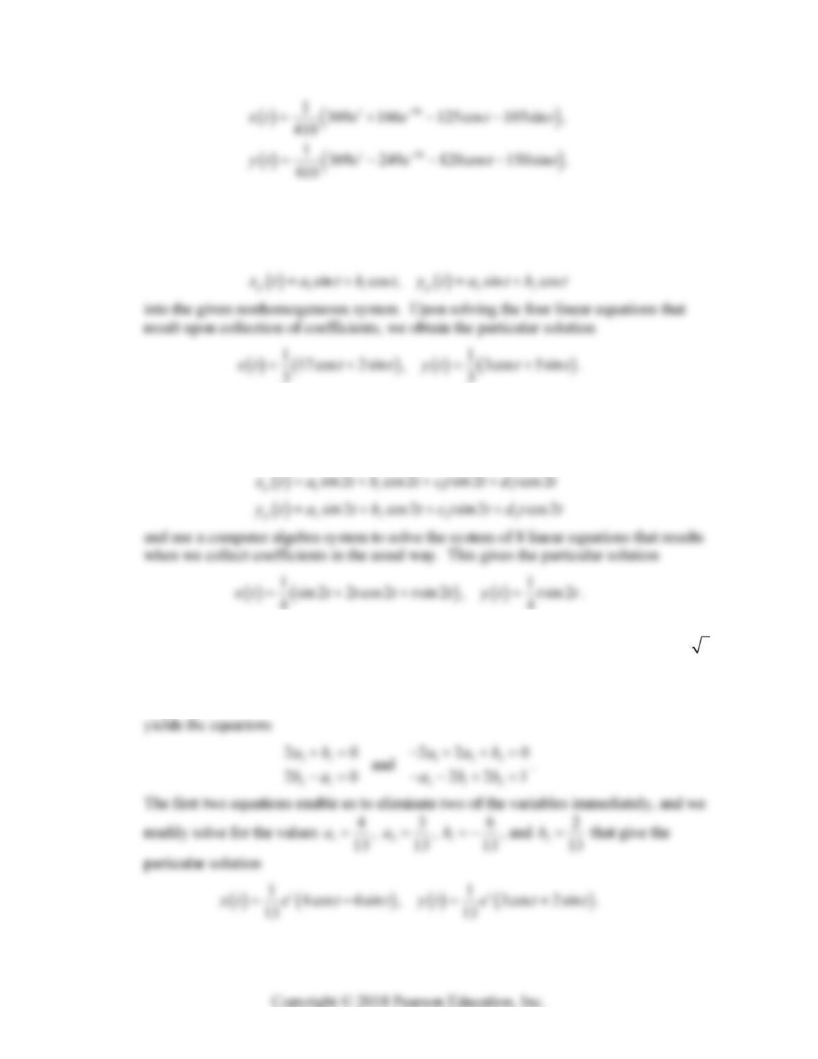
8. The coefficient matrix of the associated homogeneous system has eigenvalues 2i
,
so the complementary function involves cos2t and sin 2t. There being therefore no
duplication, we substitute the trial solution
x
9. Here the associated homogeneous system is the same as in Problem 8, so the
nonhomogeneous term cos2t duplicates the complementary function. We therefore
substitute the trial solution
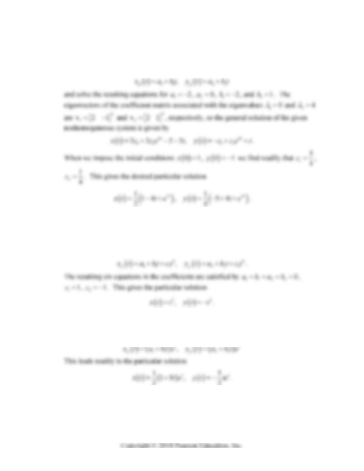
10. The coefficient matrix of the associated homogeneous system has eigenvalues 3i
,
so there is no duplication. Substitution of the trial solution
11 2 2
cos sin , cos sin
tt t t
pp
x
tae tbe tytae tbe t
Section 8.2: Nonhomogeneous Linear Systems 487
11. The coefficient matrix of the associated homogeneous system has eigenvalues 10
and
24,
so there is duplication of constant terms. We therefore substitute the particular
solution
12. The coefficient matrix of the associated homogeneous system has eigenvalues 10
and
22,
so there is duplication of constant terms in the first natural attempt. We must
multiply the t-terms by t and include all lower-degree terms in the trial solution. Thus we
substitute the trial solution
13. The coefficient matrix of the associated homogeneous system has eigenvalues 11
and
23,
so there is duplication of t
e terms. We therefore substitute the trial solution
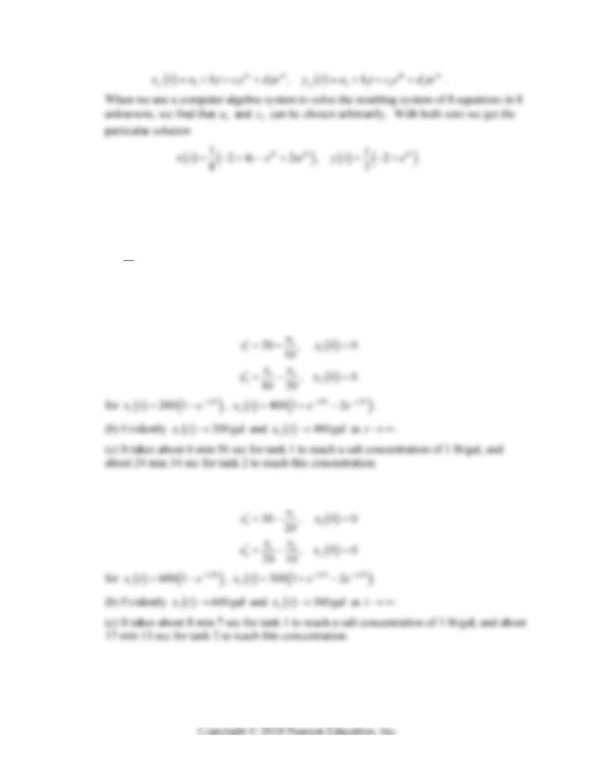
14. The coefficient matrix of the associated homogeneous system has eigenvalues 10
and
24,
so there is duplication of both constant terms and 4t
e terms. We therefore
substitute the particular solution
488 Chapter 8: Matrix Exponential Methods
x
x
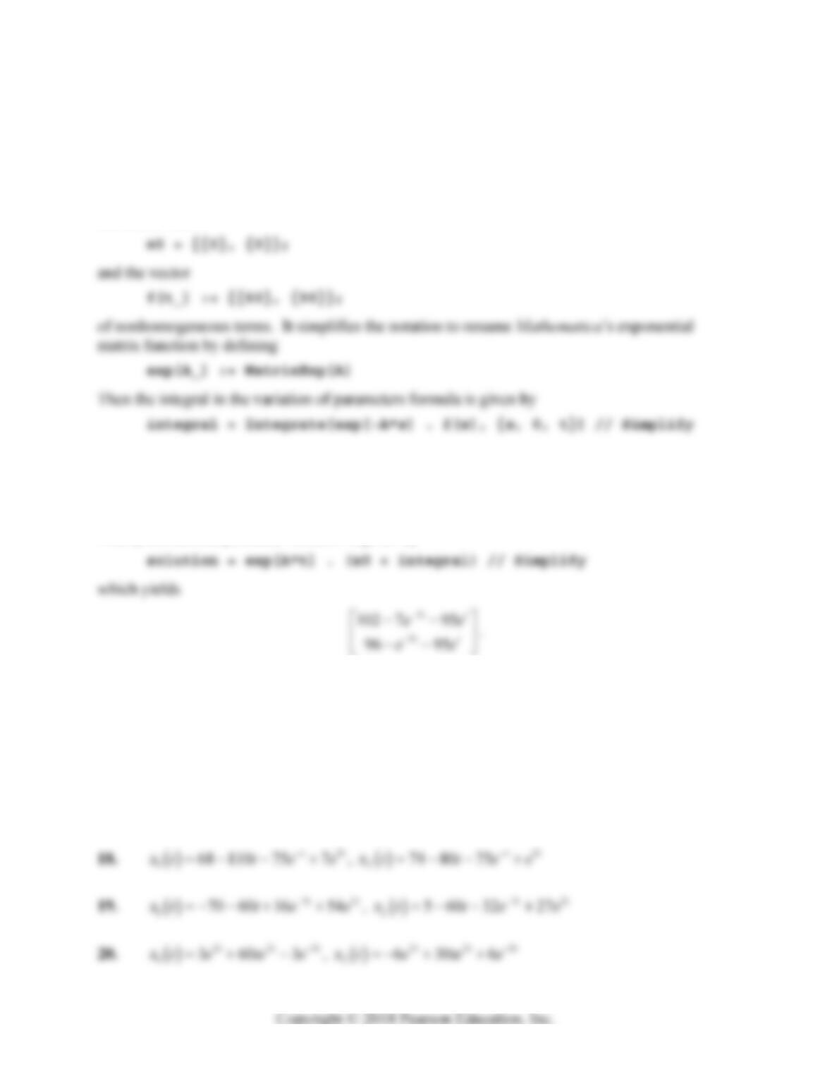
In Problems 15 and 16 the amounts
1
x
t and
2
x
t in the two tanks satisfy the equations
101121122
,
x
rc k x x k x k x
,
where i
i
r
kV
, in terms of the flow rate r, the inflowing concentration 0
c, and the volumes 1
V
and 2
V of the two tanks.
15. (a) We solve the initial value problem
16. (a) We solve the initial value problem
Section 8.2: Nonhomogeneous Linear Systems 489
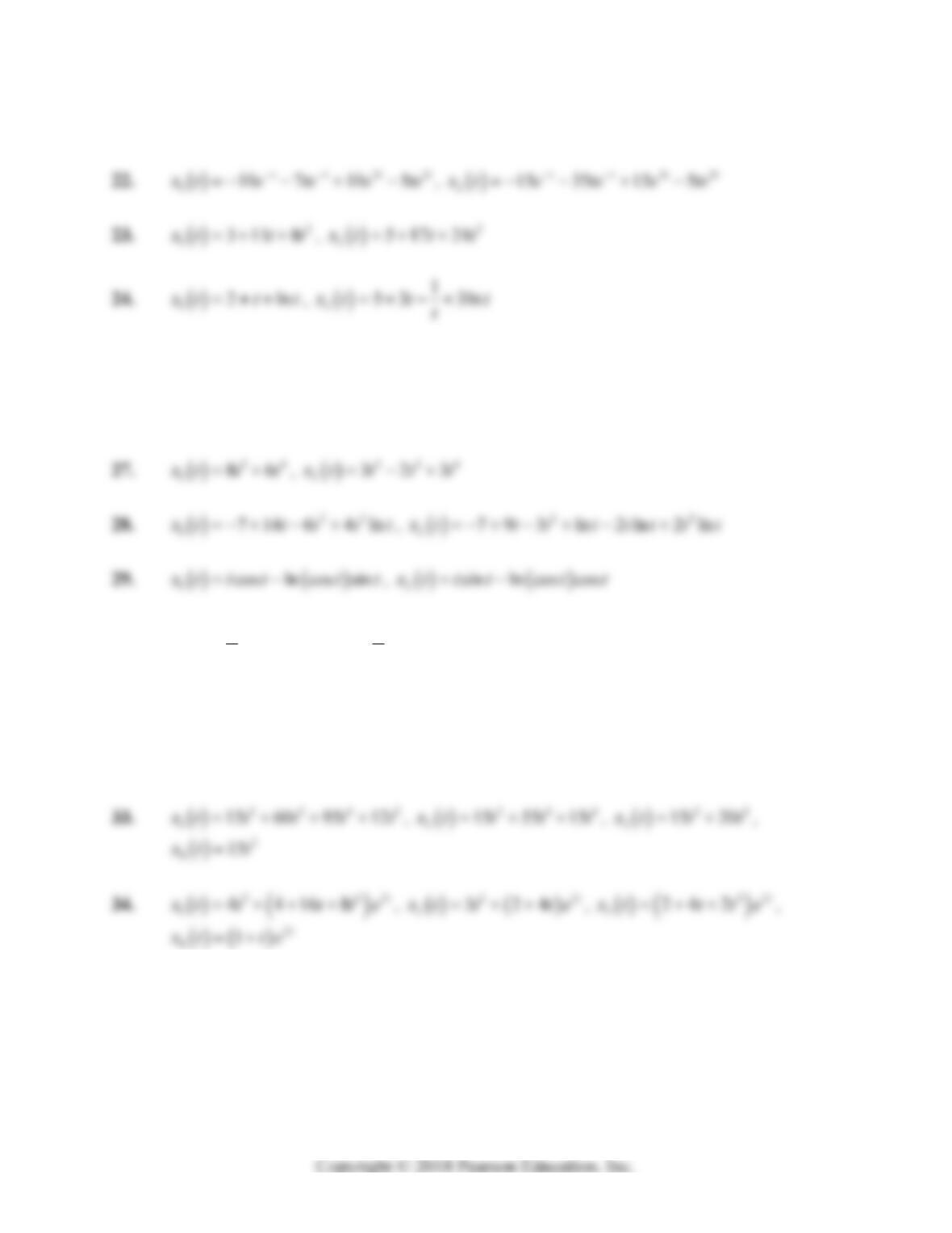
In Problems 17–34 we apply the variation of parameters formula in Eq. (28) of Section 8.2. The
answers shown below were actually calculated using the Mathematica code listed in the
application for Section 8.2. For instance, for Problem 17 we first enter the coefficient matrix
A = {{6, -7}, {1, -2}};
the initial vector
and yields the output
5
5
102 7 95
96 95
tt
tt
ee
ee
.
Finally the desired particular solution is given by
(Maple and MATLAB versions of this computation are provided in the online Extended
Applications that accompany the textbook.)
In each succeeding problem, we need only substitute the given coefficient matrix A, initial vector
x0, and the vector f of nonhomogeneous terms in the above commands, and then re-execute
them in turn. We give below only the component functions of the final results.
17.
5
1102 95 7
tt
x
tee
,
5
296 95 tt
x
tee
x
x
x
x
490 Chapter 8: Matrix Exponential Methods
21.
23
114 15
ttt
x
te e e
,
23
251015
ttt
x
teee
x
x
x
x
x
x
25.
118 cos 8sin
x
tttt ,
224 2cos 3sin
x
tttt
26.
13cos 32sin 17 cos 4 sin
x
ttttttt ,
25cos 13sin 6 cos 5 sin
x
ttttttt
x
x
x
x
x
x
30.
2
1
1cos2
2
x
tt t,
2
2
1sin 2
2
x
tt t
31.
23
194t
x
ttte ,
2
26t
x
tte,
36t
x
tte
32.
2
144 18 44 26
tt
x
tte te ,
2
2666
tt
x
te te ,
2
32t
x
tte
x
x
x
x
x
x
x
x
Section 8.3: Spectral Decomposition Methods 491
SECTION 8.3
SPECTRAL DECOMPOSITION METHODS
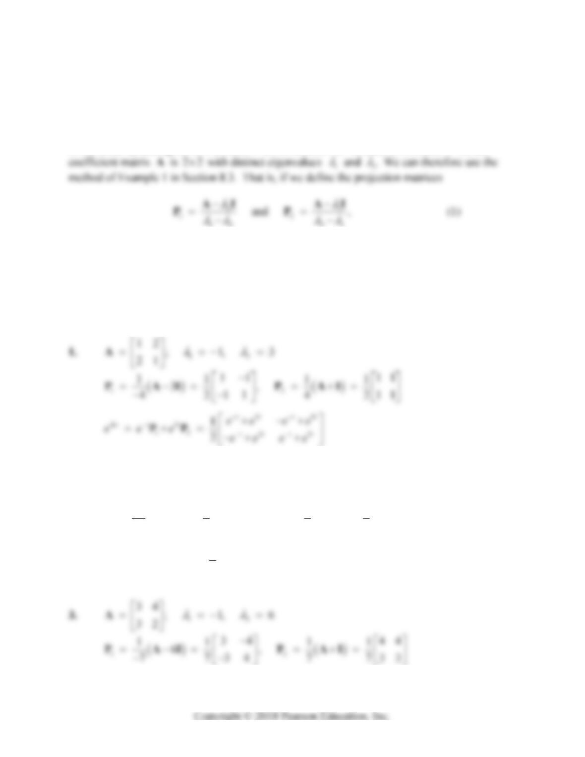
In Problems 1–20 here we want to use projection matrices to find fundamental matrix solutions
of the linear systems given in Problems 1–20 of Section 7.3. In each of Problems 1–16, the
12 21
then the desired fundamental matrix solution of the system
xAx is the exponential matrix
12
12
.
tt
t
eee
APP (2)
We use the eigenvalues 12
and
given in the Section 7.3 solutions for these problems.
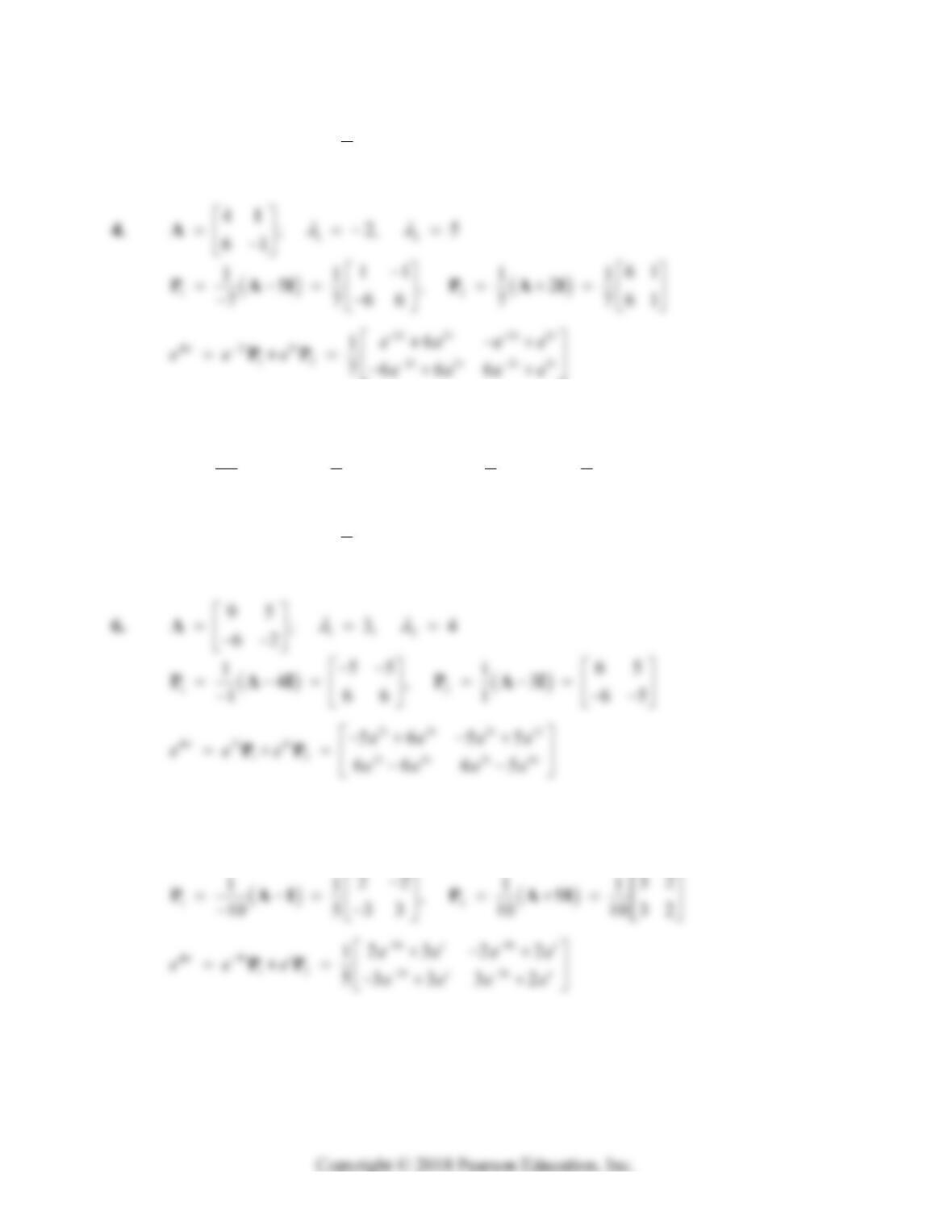
2. 12
23
;1,4
21
A
12
23 33
11 11
4,
23 22
55 55
PAI PAI
44
4
12 44
23 33
1
522 32
tt tt
tt t
tt tt
ee ee
eee ee ee
APP
492 Chapter 8: Matrix Exponential Methods
66
6
12 66
34 44
1
733 43
tt tt
ttt
tt tt
ee ee
eee ee ee
APP
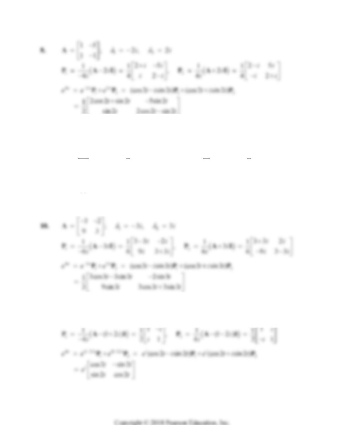
5. 12
67
;1,5
12
A
12
17 7 7
11 11
5,
17 1 1
66 66
PAI PAI
55
5
12 55
777
1
67
tt tt
ttt
tt tt
eeee
eee ee ee
APP
7. 12
34
;9,1
65
A
Section 8.3: Spectral Decomposition Methods 493
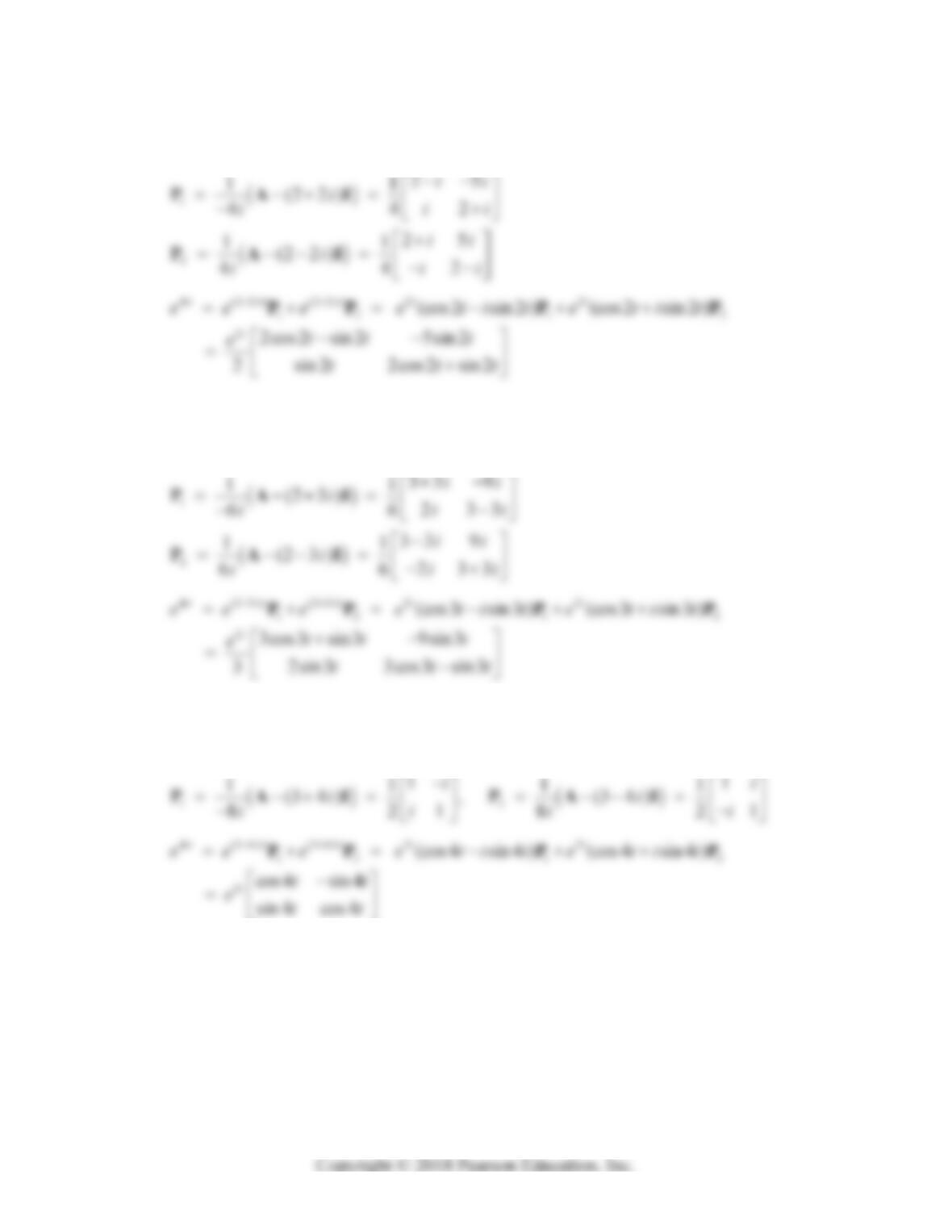
9. 12
25
;4,4
42 ii
A
12
42 5 42 5
11 11
4,4
442 442
88 88
ii ii
ii
ii ii
ii
PAI PAI
44
12 1 2
(cos 4 sin 4 ) (cos 4 sin 4 )
4cos4 2sin4 5sin4
1
4sin4 4cos4 2sin4
4
titit
ee e tit tit
tt t
ttt
APP P P
11. 12
12
;12, 12
21 ii
A
494 Chapter 8: Matrix Exponential Methods
12. 12
15
;22, 22
13 ii
A
13. 12
59
;23, 23
21 ii
A
14. 12
34
;34, 34
43 ii
A