Section 3.6: Determinants 215
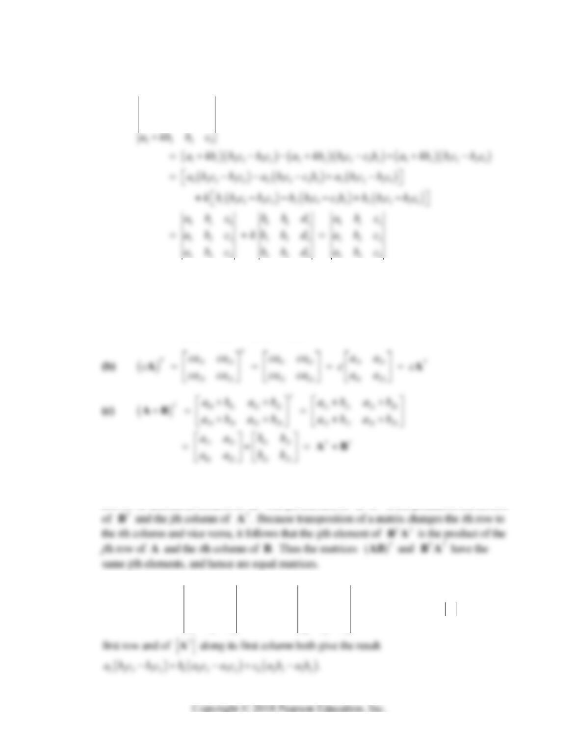
46. We expand the left-hand determinant along its first column:
1111
2222
akb bc
akbbc
47. We illustrate these properties with 22 matrices and .
ij ij
ab
AB
(a)
11 21 11 12
12 22 22 22
T
T
Taa aa
aa aa
AA
48. The ijth element of ( )T
AB is the jith element of AB, and hence is the product of the jth
row of A and the ith column of B. The ijth element of TT
BA is the product of the ith row
49. If we write
111 12 3
222 12 3
333 12 3
and ,
T
abc aaa
abc bbb
abc ccc
AA
then expansion of A along its
216 Chapter 3: Linear Systems and Matrices
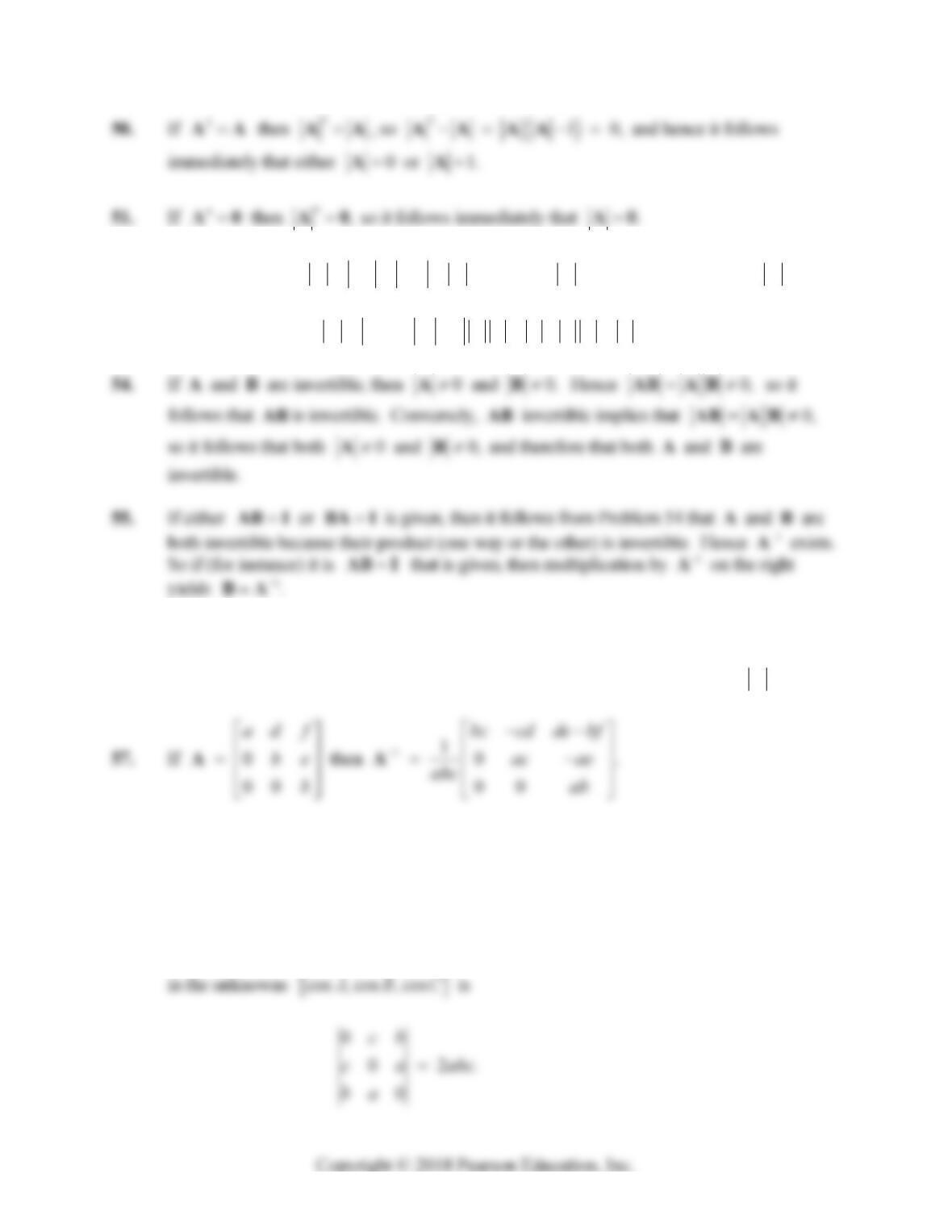
52. If 1T
AA then 1
1.
T
AA A A Hence 21,A so it follows that 1.A
53. If 1
APBP then 1
11 .
APBPPBPPBPB
56. The matrix A–1 in part (a) and the solution vector x in part (b) have only integer entries
because the only division involved in their calculation — using the adjoint formula for the
inverse matrix or Cramer’s rule for the solution vector — is by the determinant 1.A
58. The coefficient determinant of the linear system
cos cos
cos cos
cos cos
cBbCa
cA aCb
bAaB c
Section 3.6: Determinants 217
59. These are almost immediate computations.
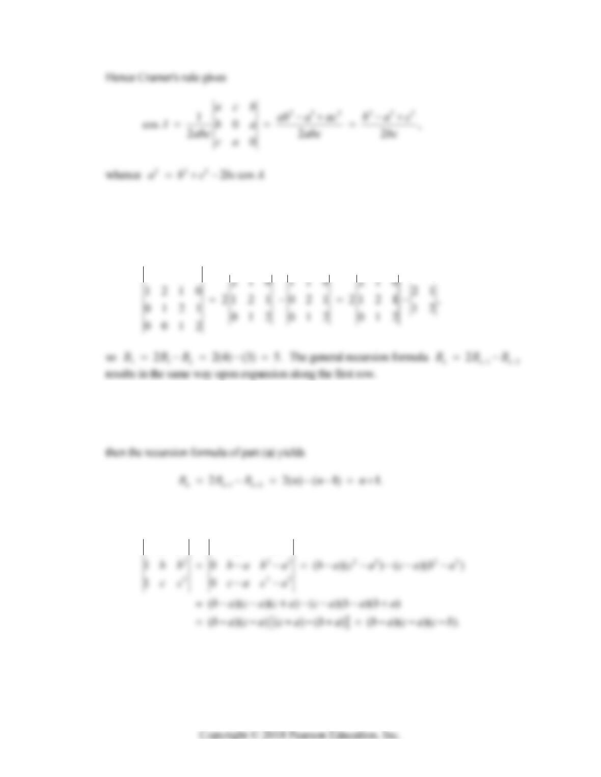
60. (a) In the 4 4 case, expansion along the first row gives
2100 210 110 210
(b) If we assume inductively that
12
(1)1 and (2)1 1,
nn
Bn nB n n
61. Subtraction of the first row from both the second and the third row gives
22
11
aa a a
218 Chapter 3: Linear Systems and Matrices
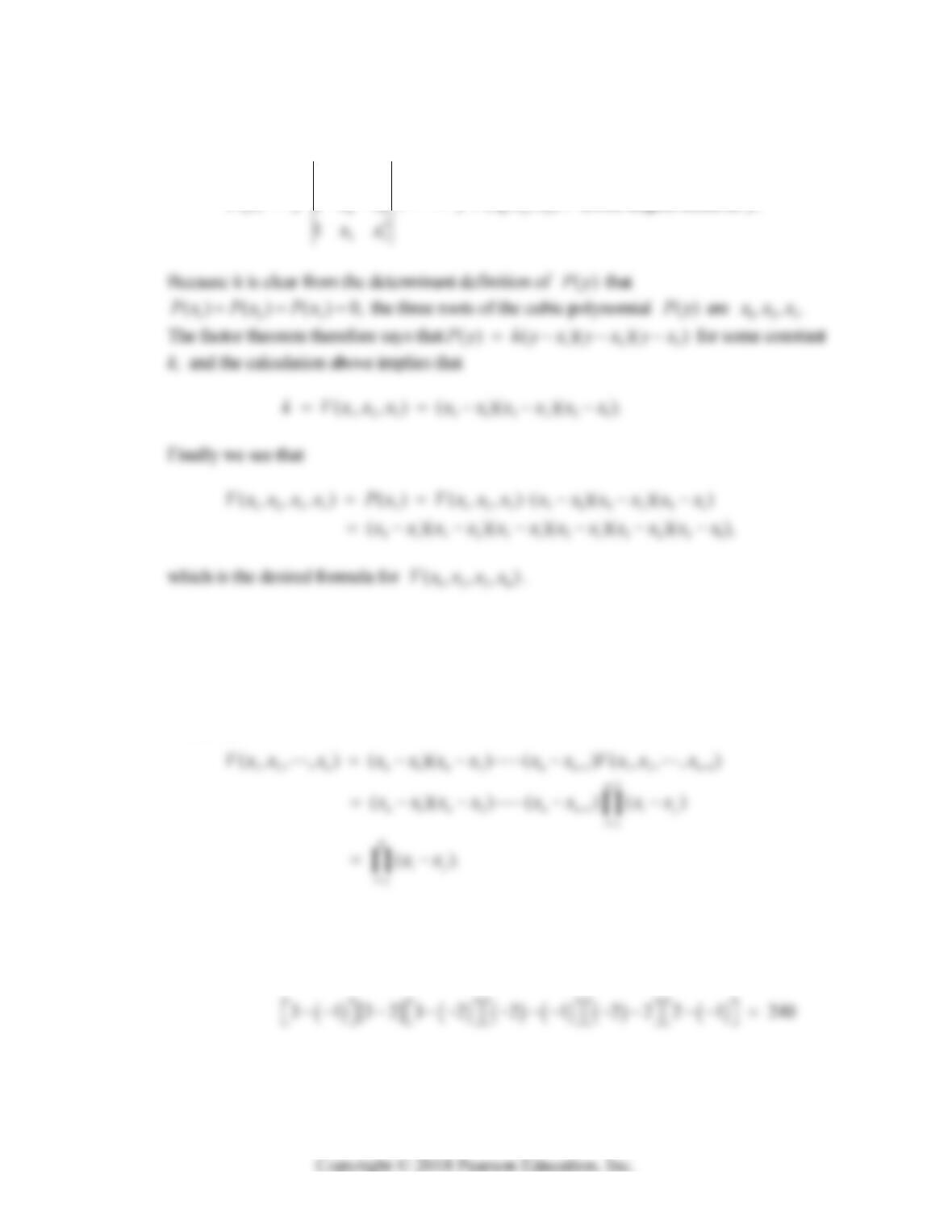
62. Expansion of the 4 4 determinant defining ( )Py along its 4th row yields
2
11
32 3
1
() 1 ( , , )
xx
Py y x x yVx x x
lower-degree terms in y.
63. The same argument as in Problem 62 yields
12 1 1 2 1
() ( , , , )( )( ) ( ).
nn
Py Vxx x yx yx yx
Therefore
64. (a) V(1, 2, 3, 4) = (4 – 1)(4 – 2)(4 – 3)(3 – 1)(3 – 2)(2 – 1) = 12
(b) V(–1, 2,–2, 3) =
Section 3.7: Linear Equations and Curve Fitting 219
SECTION 3.7
LINEAR EQUATIONS AND CURVE FITTING
In Problems 1–10 we first set up the linear system in the coefficients , ,ab that we get by
substituting each given point
(, )
ii
x
y
into the desired interpolating polynomial equation
.yabx Then we give the polynomial that results from solution of this linear system.
1. ()
y
xabx
11 1 2, 3 so ( ) 2 3
13 7
aab yx x
b
y
y
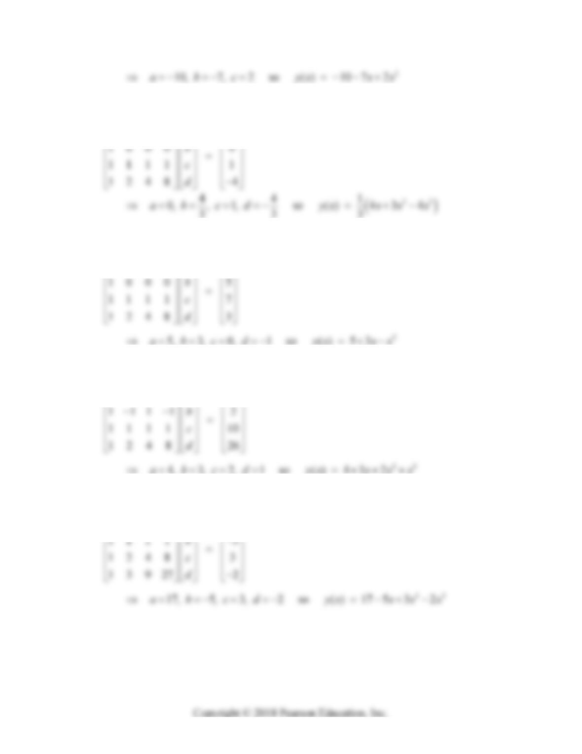
4. 2
()
y
xabxcx
2
111 1
111 5 0, 2, 3 so () 2 3
124 16
a
babcyxxx
c
5. 2
()
y
xabxcx
111 3
a
6. 2
()
y
xabxcx
111 1
a
220 Chapter 3: Linear Systems and Matrices
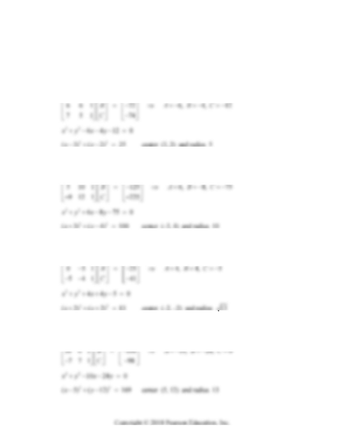
7. 23
()
y
x a bx cx dx
1111 1
a
8. 23
()
y
x a bx cx dx
1111 3
a
9. 23
()
y
x a bx cx dx
1248 2
a
10. 23
()
y
x a bx cx dx
111 1 17
a
Section 3.7: Linear Equations and Curve Fitting 221
In Problems 11–14 we first set up the linear system in the coefficients , ,ABC that we get by
substituting each given point
(, )
ii
x
y
into the circle equation 22
Ax By C x y (see
Eq. (9) in the text). Then we give the circle that results from solution of this linear system.
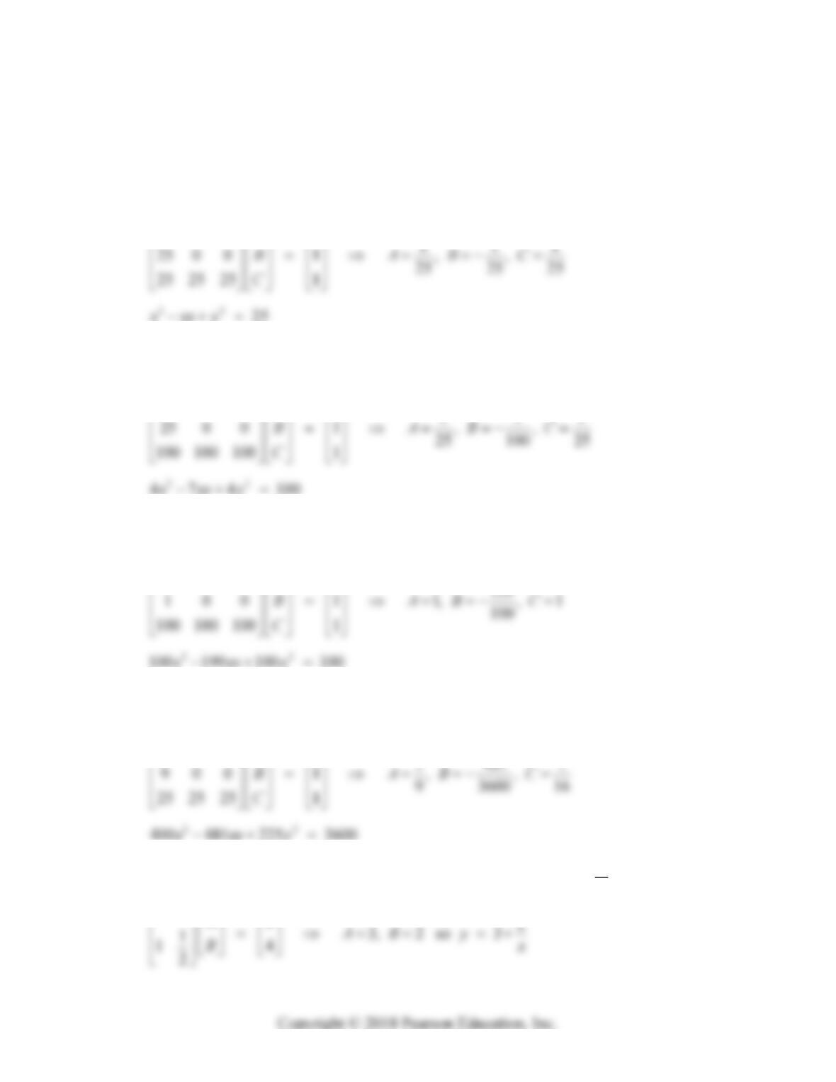
11. 22
Ax By C x y
111 2
A
12. 22
Ax By C x y
341 25
A
13. 22
Ax By C x y
101 1
A
14. 22
Ax By C x y
001 0
A
222 Chapter 3: Linear Systems and Matrices
In Problems 15–18 we first set up the linear system in the coefficients , ,ABC that we get by
substituting each given point
(, )
ii
x
y
into the central conic equation 22
1Ax Bxy Cy (see
Eq. (10) in the text). Then we give the equation that results from solution of this linear system.
15. 22
1Ax Bxy Cy
0025 1 111
A
16. 22
1Ax Bxy Cy
0025 1 171
A
17. 22
1Ax Bxy Cy
001 1 199
A
18. 22
1Ax Bxy Cy
0016 1 1 481 1
A
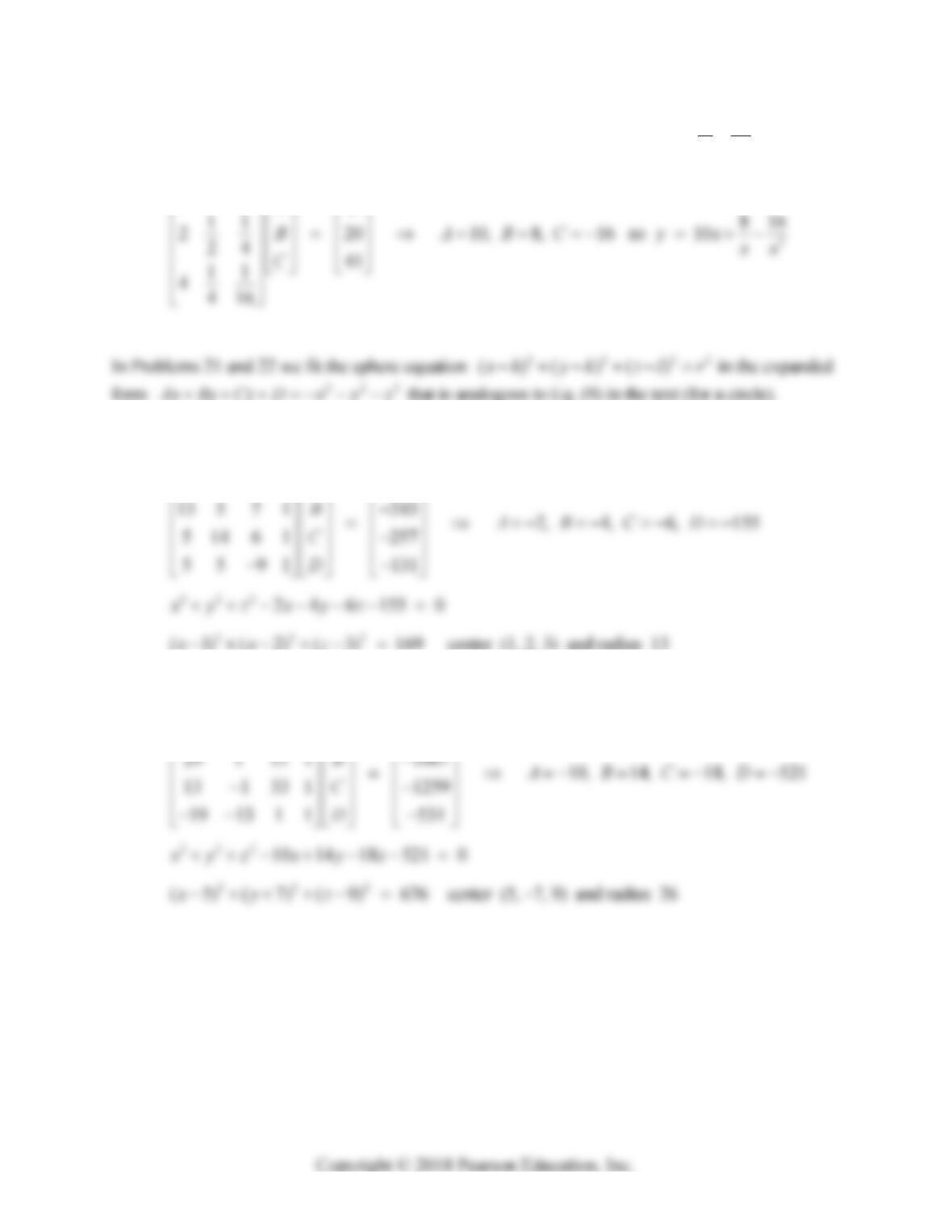
19. We substitute each of the two given points into the equation
B
yA
x
.
11 52
AAB y
Section 3.7: Linear Equations and Curve Fitting 223
20. We substitute each of the three given points into the equation 2
B
C
yAx
x
x
:
x
x
11 1 2
A
21. 222
Ax By Cz D x y z
4 6 15 1 277
A
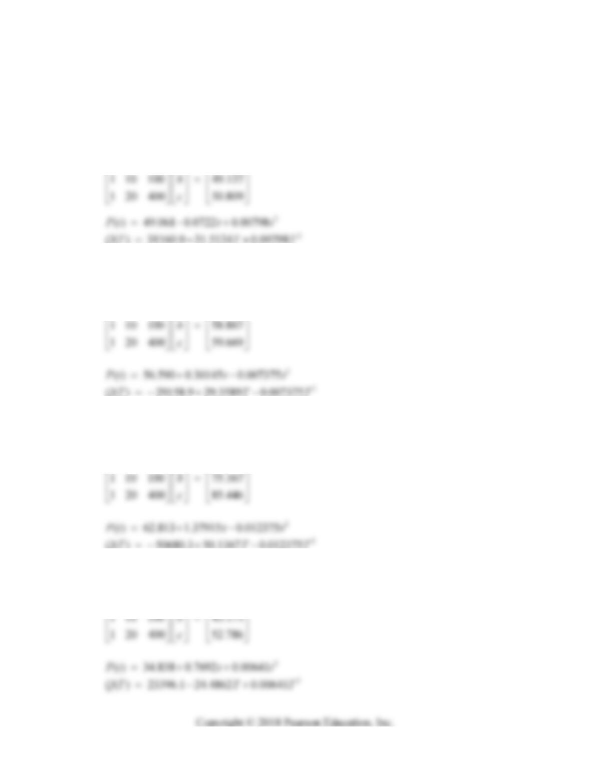
22. 222
Ax By Cz D x y z
11 17 17 1 699
A
224 Chapter 3: Linear Systems and Matrices
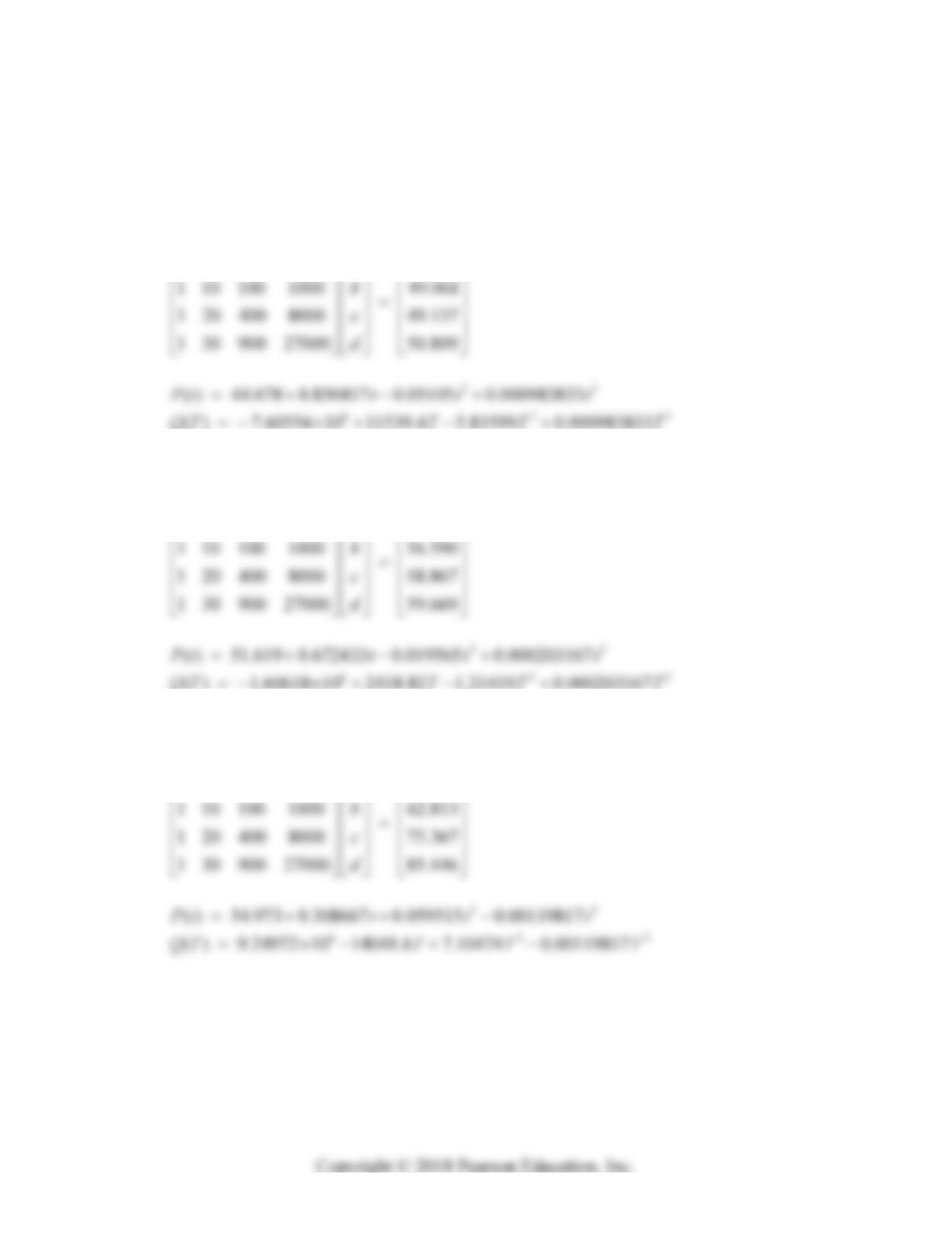
In Problems 23–26 we first take t = 0 in 1970 to fit a quadratic polynomial 2
() .Pt a bt ct
Then we write the quadratic polynomial ( ) ( 1970)QT PT that expresses the predicted
population in terms of the actual calendar year T.
23. 2
()Pt a bt ct
1 0 0 49.061
a
24. 2
()Pt a bt ct
1 0 0 56.590
a
25. 2
()Pt a bt ct
1 0 0 62.813
a
26. 2
()Pt a bt ct
1 0 0 34.838
a
Section 3.7: Linear Equations and Curve Fitting 225
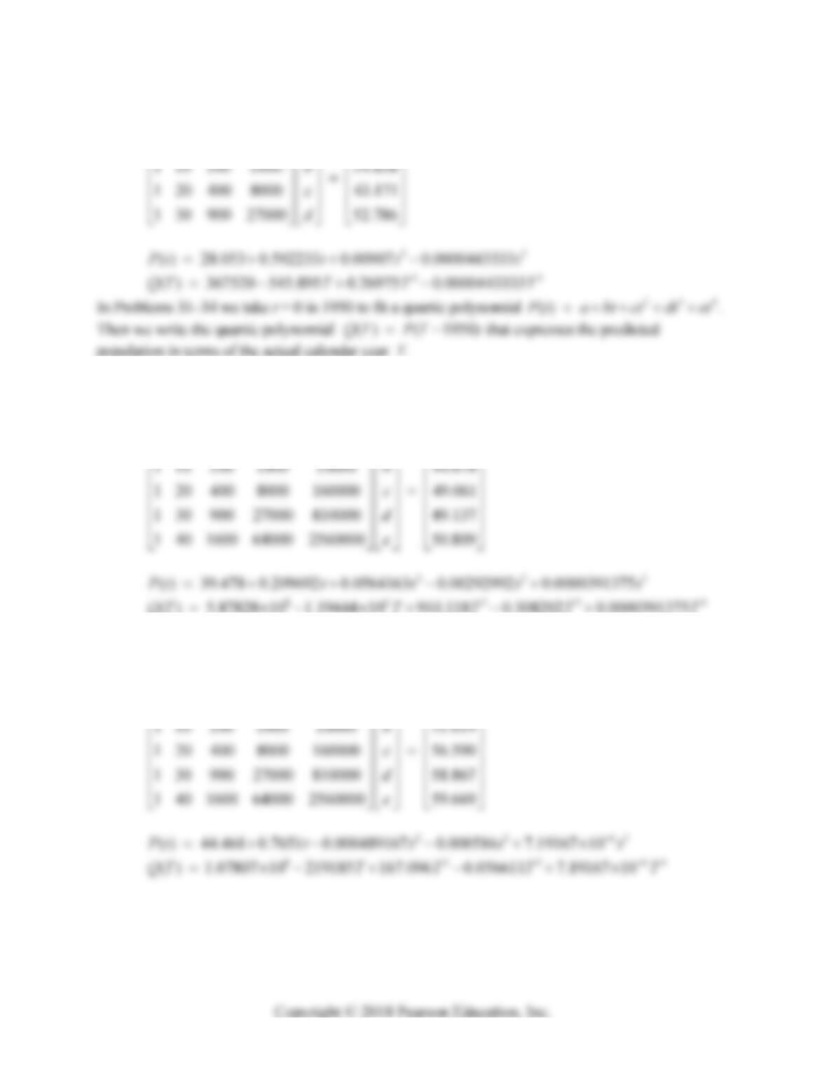
In Problems 27–30 we first take t = 0 in 1960 to fit a cubic polynomial 23
() .Pt a bt ct dt
Then we write the cubic polynomial ( ) ( 1960)QT PT that expresses the predicted population
in terms of the actual calendar year T.
27. 23
()Pt a bt ct dt
1 0 0 0 44.678
a
28. 23
()Pt a bt ct dt
1 0 0 0 51.619
a
29. 23
()Pt a bt ct dt
1 0 0 0 54.973
a
226 Chapter 3: Linear Systems and Matrices
30. 23
()Pt a bt ct dt
1 0 0 0 28.053
a
31. 234
() .Pt a bt ct dt et
1 0 0 0 0 39.478
a
32. 234
() .Pt a bt ct dt et
1 0 0 0 0 44.461
a
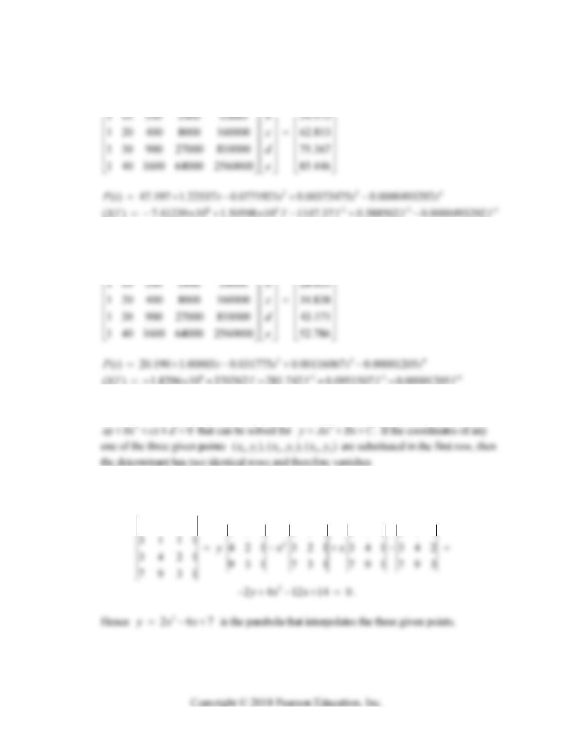
Section 3.7: Linear Equations and Curve Fitting 227
33. 234
() .Pt a bt ct dt et
1 0 0 0 0 47.197
a
34. 234
() .Pt a bt ct dt et
1 0 0 0 0 20.190
a
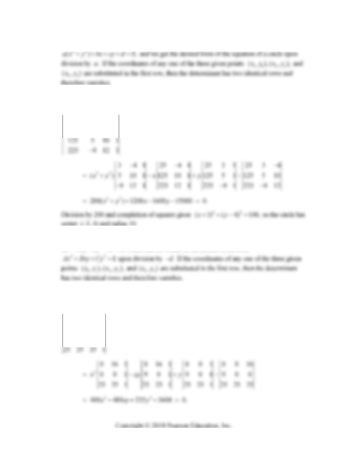
35. Expansion of the determinant along the first row gives an equation of the form
36. Expansion of the determinant along the first row gives
2
1111 311 311 311
yx x
228 Chapter 3: Linear Systems and Matrices
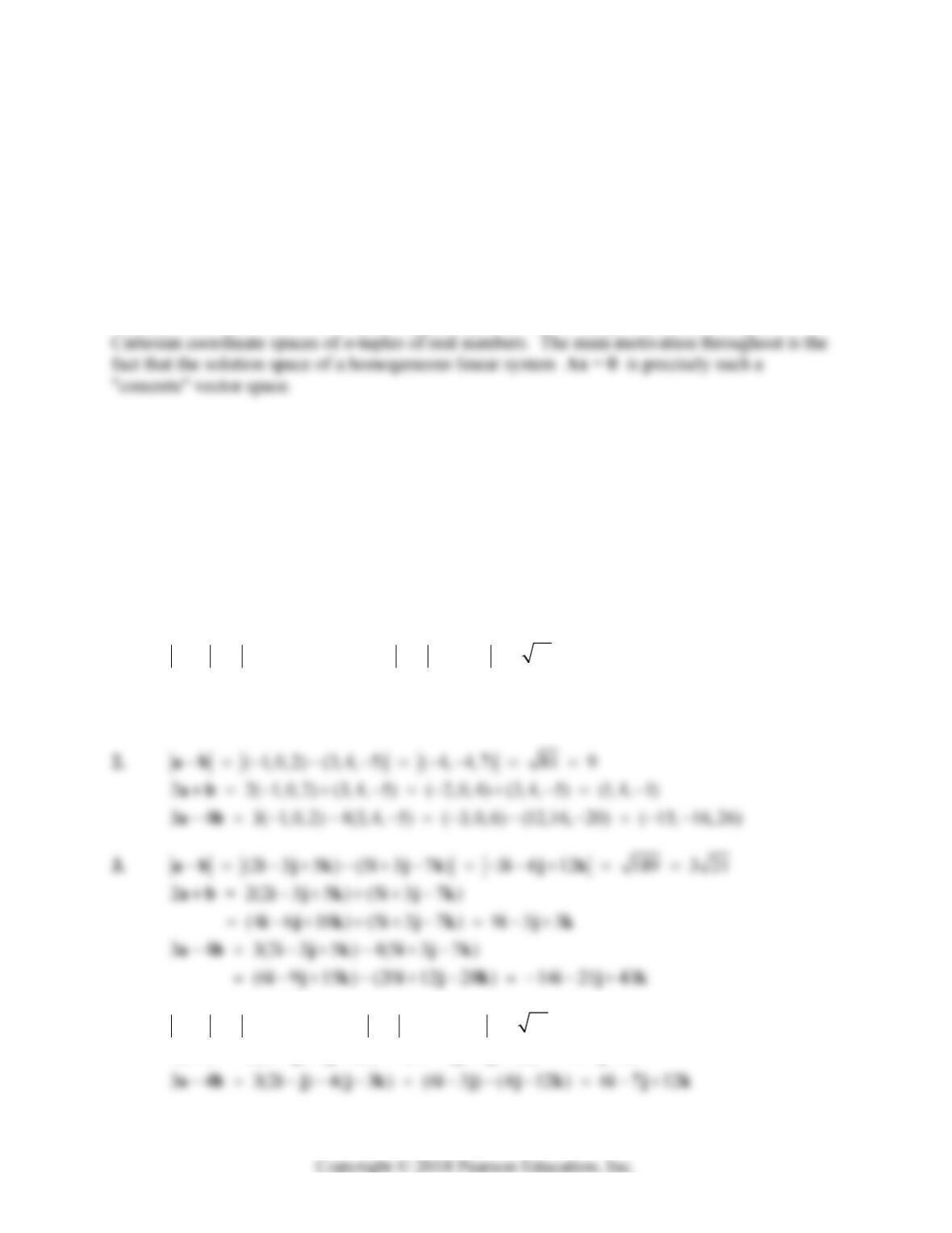
37. Expansion of the determinant along the first row gives an equation of the form
38. Expansion of the determinant along the first row gives
22 1
25 3 4 1
xy x y
39. Expansion of the determinant along the first row gives an equation of the form
22
0,ax bxy cy d which can be written in the central conic form
40. Expansion of the determinant along the first row gives
22
1
00161
9001
xxyy
229
CHAPTER 4
VECTOR SPACES
The treatment of vector spaces in this chapter is very concrete. Prior to the final section of the
chapter, almost all of the vector spaces appearing in examples and problems are subspaces of
SECTION 4.1
THE VECTOR SPACE R3
Here the fundamental concepts of vectors, linear independence, and vector spaces are introduced in
the context of the familiar 2-dimensional coordinate plane R2 and 3-space R3. The concept of a
subspace of a vector space is illustrated, the proper nontrivial subspaces of R3 being simply lines
and planes through the origin.
1. (2,5, 4) (1, 2, 3) (1,7, 1) 51 ab
2 2(2, 5, 4) (1, 2, 3) (4,10, 8) (1, 2, 3) (5,8, 11)
3 4 3(2,5, 4) 4(1, 2, 3) (6,15, 12) (4, 8, 12) (2, 23, 0)
ab
ab
4. (2 ) ( 3 ) 2 2 3 17 ab ij j k i j k
ab i
jj
ki
jj
ki
j
k
230 Chapter 4: Vector Spaces
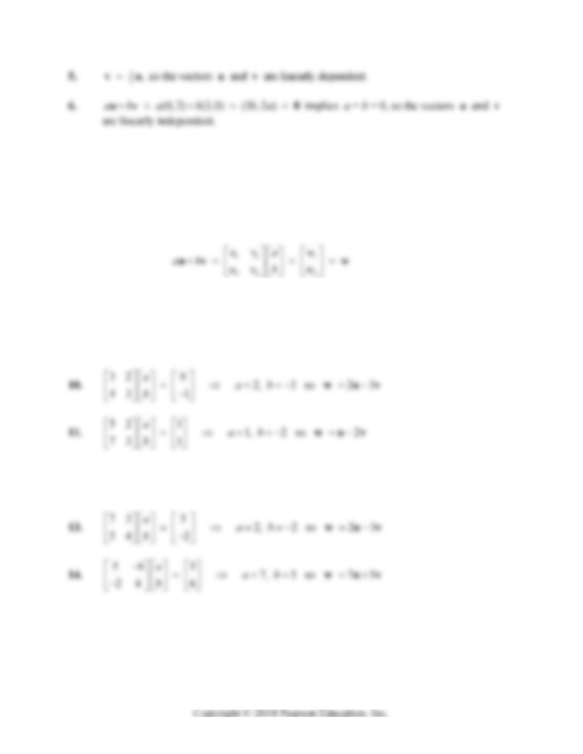
7. (2,2) (2, 2) (2 2 , 2 2 )ab a b abab uv 0 implies a = b = 0, so the vectors
u and v are linearly independent.
8. ,vu so the vectors u and v are linearly dependent.
In each of Problems 9–14, we set up and solve (as in Example 2 of this section) the system
to find the coefficient values a and b such that ,abwuv
9. 11 1 3, 2 so 3 2
23 0
aab
b
wuv
12. 42 2 3, 5 so 3 5
11 2
aab
b
wuv
Section 4.1: The Vector Space
3
R 231
In Problems 15–18, we calculate the determinant uvw so as to determine (using Theorem
4) whether the three vectors u, v, and w are linearly dependent (det = 0) or linearly
independent (det 0).
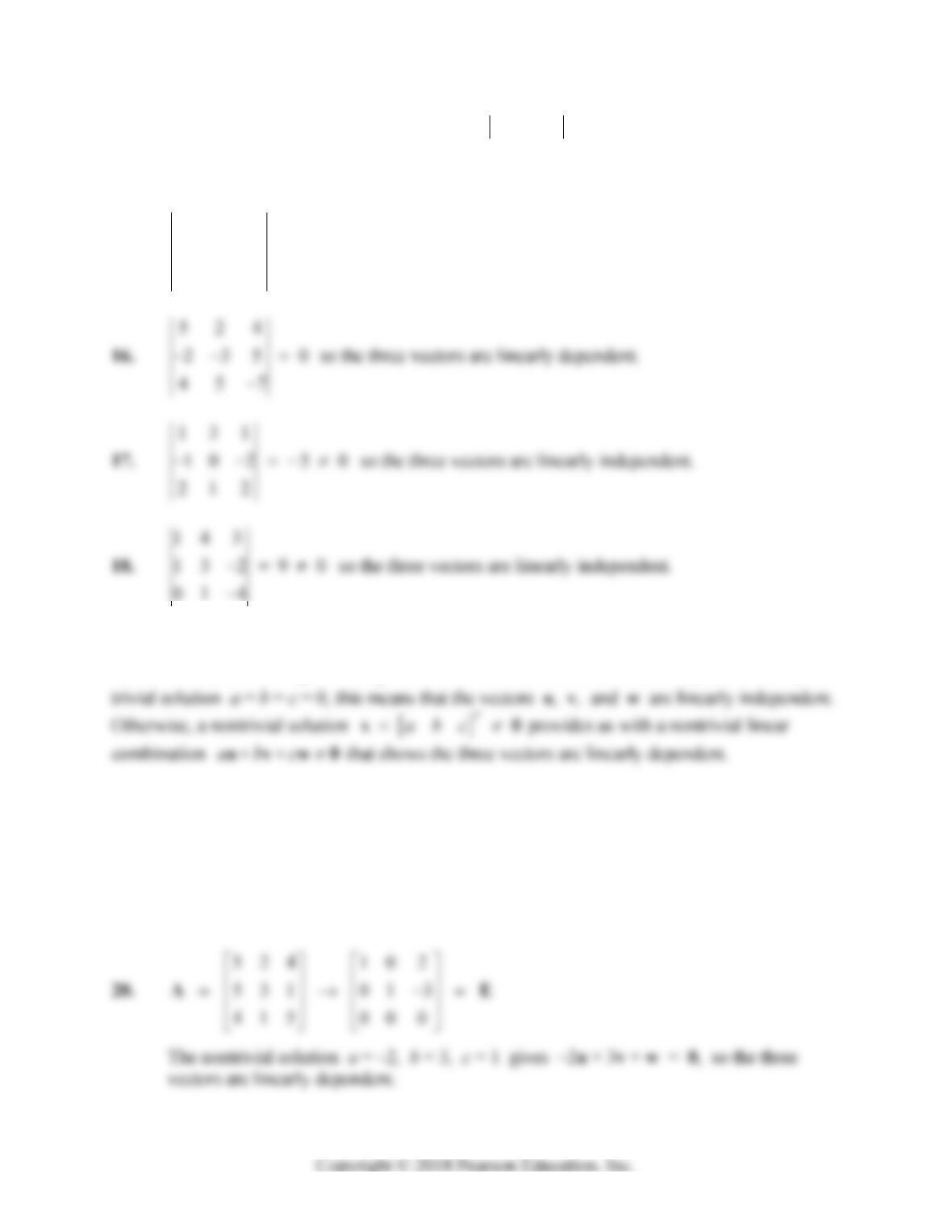
15.
358
14 3 0
264
so the three vectors are linearly dependent.
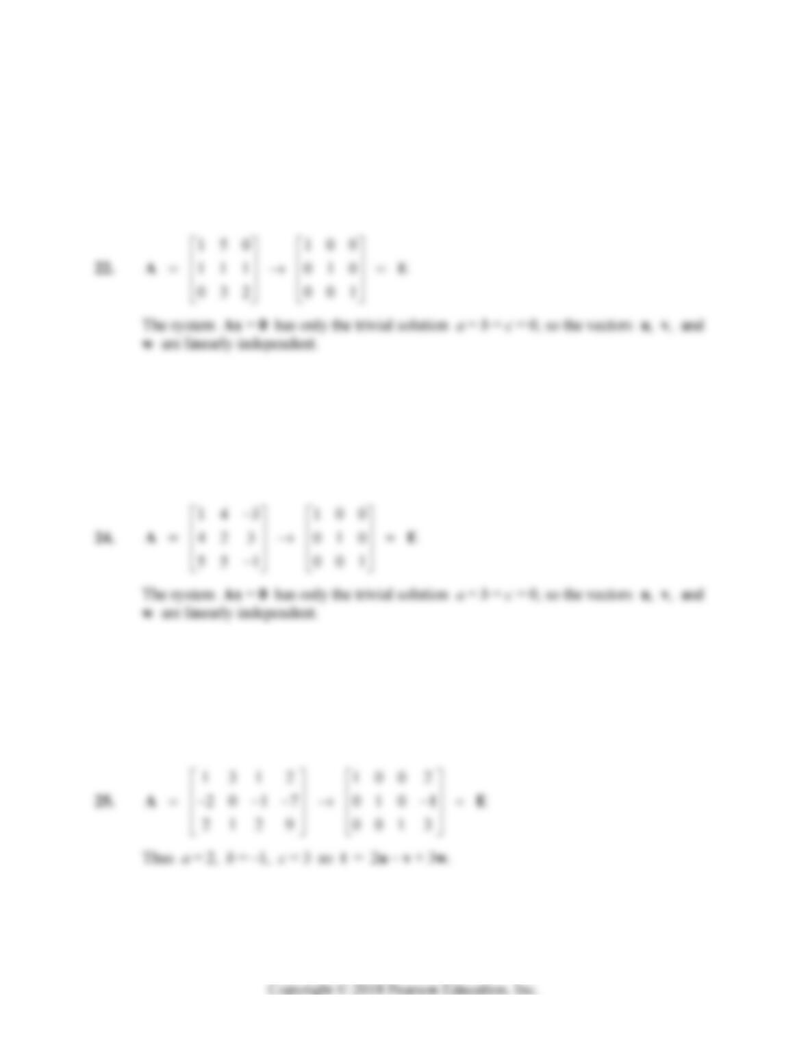
In Problems 19–24, we attempt to solve the homogeneous system Ax 0 by reducing the
coefficient matrix
Auvw to echelon form E. If we find that the system has only the
19.
230 103
01 2 01 2
111 000
AE
The nontrivial solution a = 3, b = 2, c = 1 gives 3u + 2v + w = 0, so the three vectors
are linearly dependent.
232 Chapter 4: Vector Spaces
21.
123 1011
117 014
262 000
AE
The nontrivial solution a = 11, b = 4, c = –1 gives 11u + 4v – w = 0, so the three
vectors are linearly dependent.
23.
25 2 100
04 1 010
321 001
AE
The system Ax = 0 has only the trivial solution a = b = c = 0, so the vectors u, v, and
w are linearly independent.
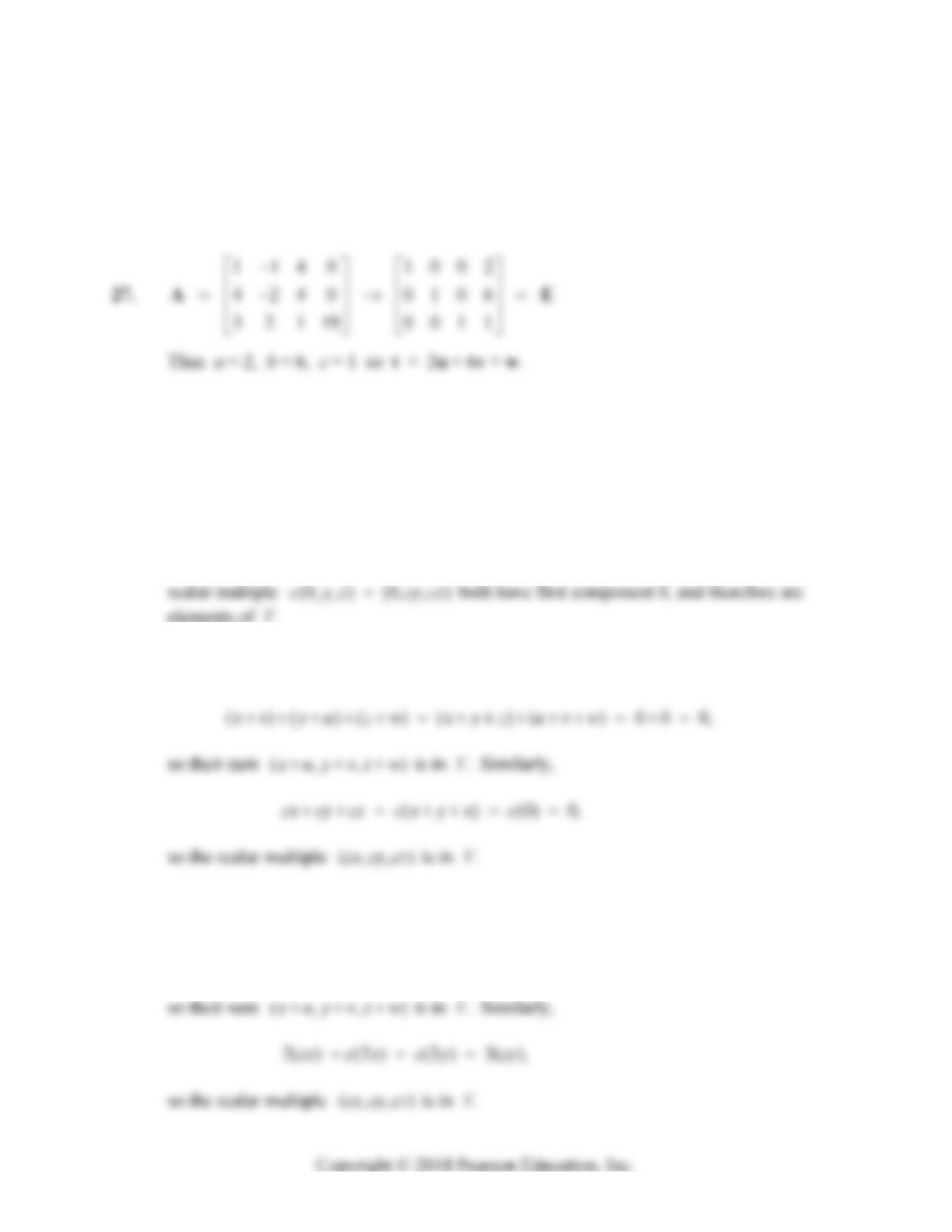
In Problems 25–28, we solve the nonhomogeneous system Ax t by reducing the augmented
coefficient matrix
Auvwt to echelon form E. The solution vector
T
abcx appears as the final column of E, and provides us with the desired linear
combination .abctuvw
Section 4.1: The Vector Space
3
R 233
26.
515 5 1001
25 330 0105
234 21 0011
AE
Thus a = 1, b = 5, c = –1 so t = u + 5v – w.
28.
2417 1001
5 1 17 0101
3157 0011
AE
Thus a = 1, b = 1, c = 1 so t = u + v + w.
29. Given vectors (0, , ) and (0, , )
y
zvw in V, we see that their sum (0, , )
y
vz w and the
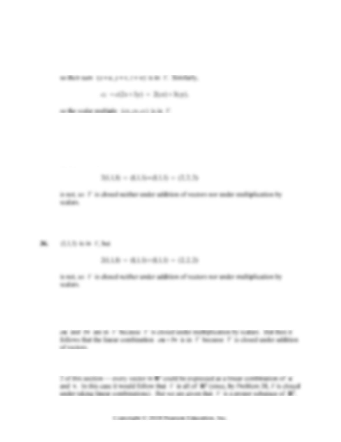
30. If ( , , ) and ( , , )
x
yz uvw are in V, then
x
31. If (, ,)and(,, )
x
yz uvw are in V, then
2( )(2)(2)(3)(3)3( ),
x
uxuyvyv
x
234 Chapter 4: Vector Spaces
32. If ( , , ) and ( , , )
x
yz uvw are in V, then
(2 3 ) (2 3 ) 2( ) 3( ),
zw x y u v xu yv
x
33. (0,1,0) is in V but the sum (0,1,0) (0,1,0) (0,2,0) is not in V; thus V is not
closed under addition. Alternatively, 2(0,1, 0) (0, 2, 0) is not in V, so V is not
closed under multiplication by scalars.
34. (1,1,1) is in V, but
35. Evidently V is closed under addition of vectors. However, (0, 0,1) is in V but
(1)(0,0,1) (0,0, 1) is not, so V is not closed under multiplication by scalars.
37. Pick a fixed element u in the (nonempty) vector space V. Then, with c = 0, the scalar
multiple 0cuu0 must be in V. Thus V necessarily contains the zero vector 0.
38. Suppose u and v are vectors in the subspace V of R3 and a and b are scalars. Then
39. It suffices to show that every vector v in V is a scalar multiple of the given nonzero
vector u in V. If u and v were linearly independent, then — as illustrated in Example