PROBLEM 4.1
KNOWN: Method of separation of variables for two–dimensional, steady-state conduction.
FIND: Show that negative or zero values of λ2, the separation constant, result in solutions which
cannot satisfy the boundary conditions.
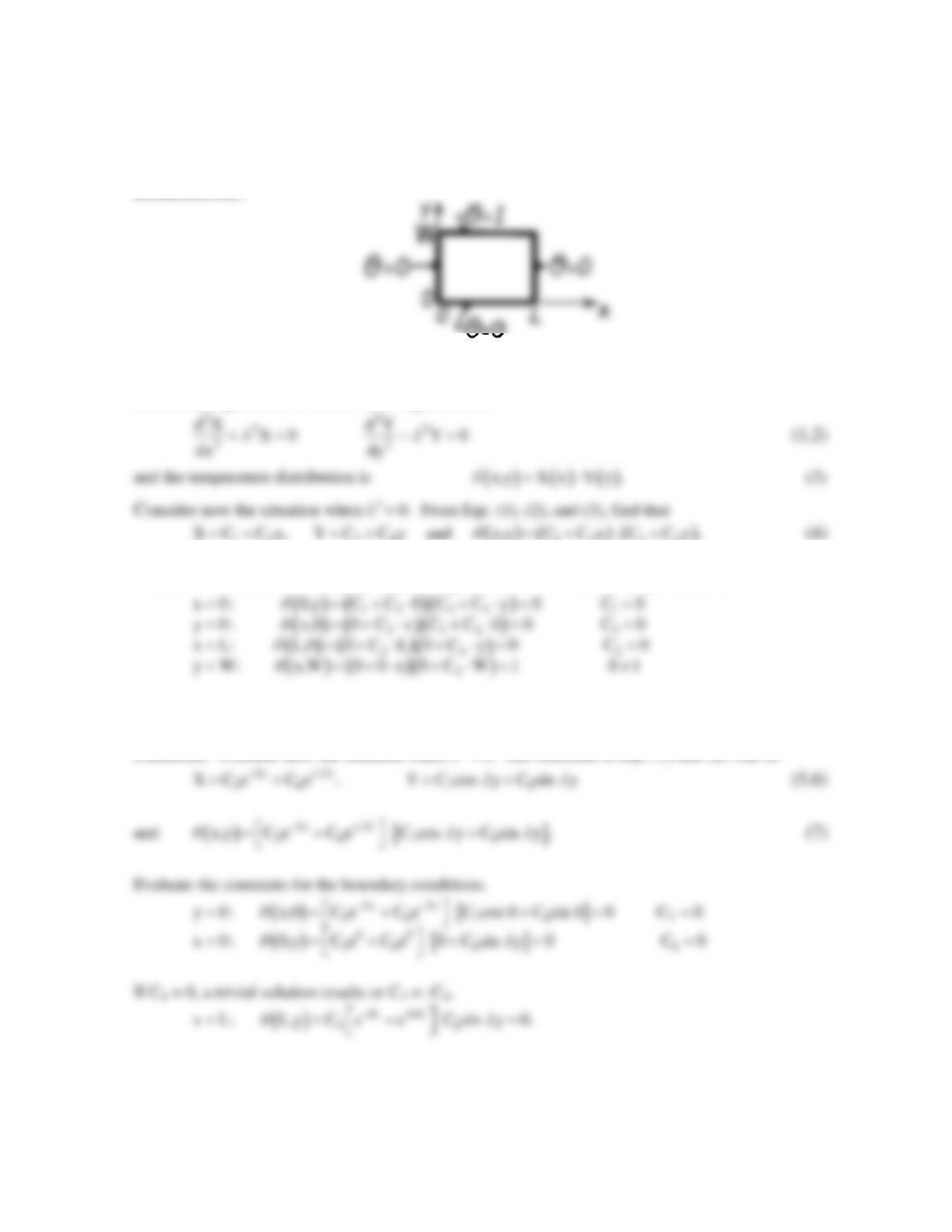
SCHEMATIC:
ASSUMPTIONS: (1) Two-dimensional, steady-state conduction, (2) Constant properties.
ANALYSIS: From Section 4.2, identification of the separation constant λ2 leads to the two ordinary
differential equations, 4.6 and 4.7, having the forms
12 34 12 34
Evaluate the constants – C1, C2, C3 and C4 – by substitution of the boundary conditions:
The last boundary condition leads to an impossibility (0 ≠ 1). We therefore conclude that a λ2 value
of zero will not result in a form of the temperature distribution which will satisfy the boundary
conditions. Consider now the situation when λ2 < 0. The solutions to Eqs. (1) and (2) will be
From the last boundary condition, we require C5 or C8 is zero; either case leads to a trivial solution
with either no x or y dependence.
PROBLEM 4.2
KNOWN: Two-dimensional rectangular plate subjected to prescribed uniform temperature boundary
conditions.
FIND: Temperatures along the mid-plane at y = 0.25, 0.5, and 0.75 m considering the first five non-zero
terms; assess error resulting from using only first three terms.
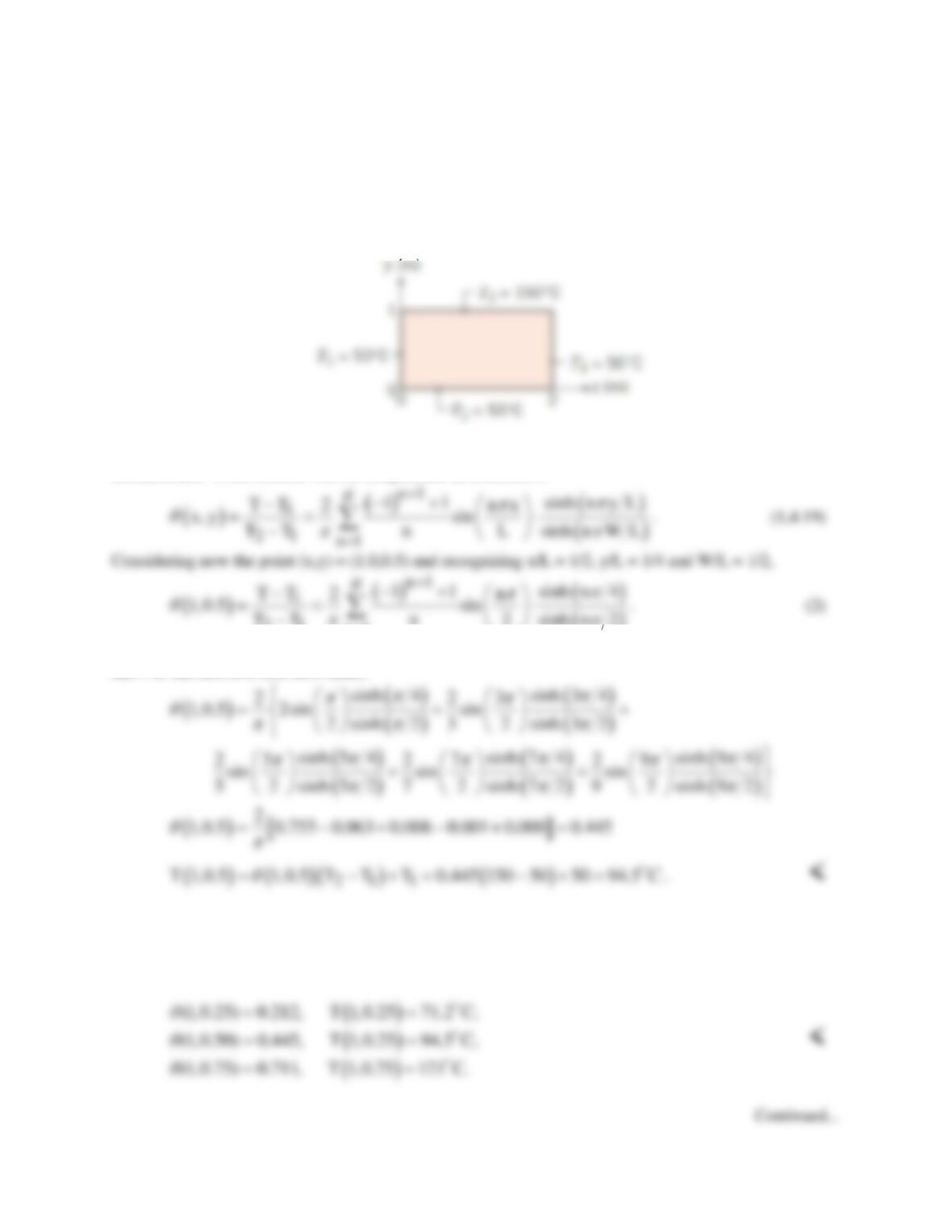
SCHEMATIC:
ASSUMPTIONS: (1) Two-dimensional, steady-state conduction, (2) Constant properties.
ANALYSIS: From Section 4.2, the temperature distribution is
( )
21 n1
T T n 2 sinh n 2
=
−
When n is even (2, 4, 6 …), the corresponding term is zero; hence we need only consider n = 1, 3, 5, 7
and 9 as the first five non-zero terms.
Repeating the calculation for y = 0.25 and 0.75 m, the only thing that changes is y/L = 1/8 and 3/8
respectively in the sinh term in the numerator. The results are (repeating the above result for
completeness):
PROBLEM 4.2 (Cont.)
If only the first three terms of the series, Eq. (2), are considered, the results are:
COMMENTS: The number of terms needed for an accurate result depends on the location, with more
terms need near those corners where there is a discontinuous change in temperature.
PROBLEM 4.3
KNOWN: Temperature distribution in the two-dimensional rectangular plate of Problem 4.2.
FIND: Expression for the heat rate per unit thickness from the lower surface (0 ≤ x ≤ 2, 0) and result
based on first five non-zero terms of the infinite series.
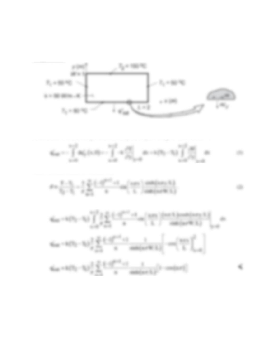
SCHEMATIC:
ASSUMPTIONS: (1) Two-dimensional, steady-state conduction, (2) Constant properties.
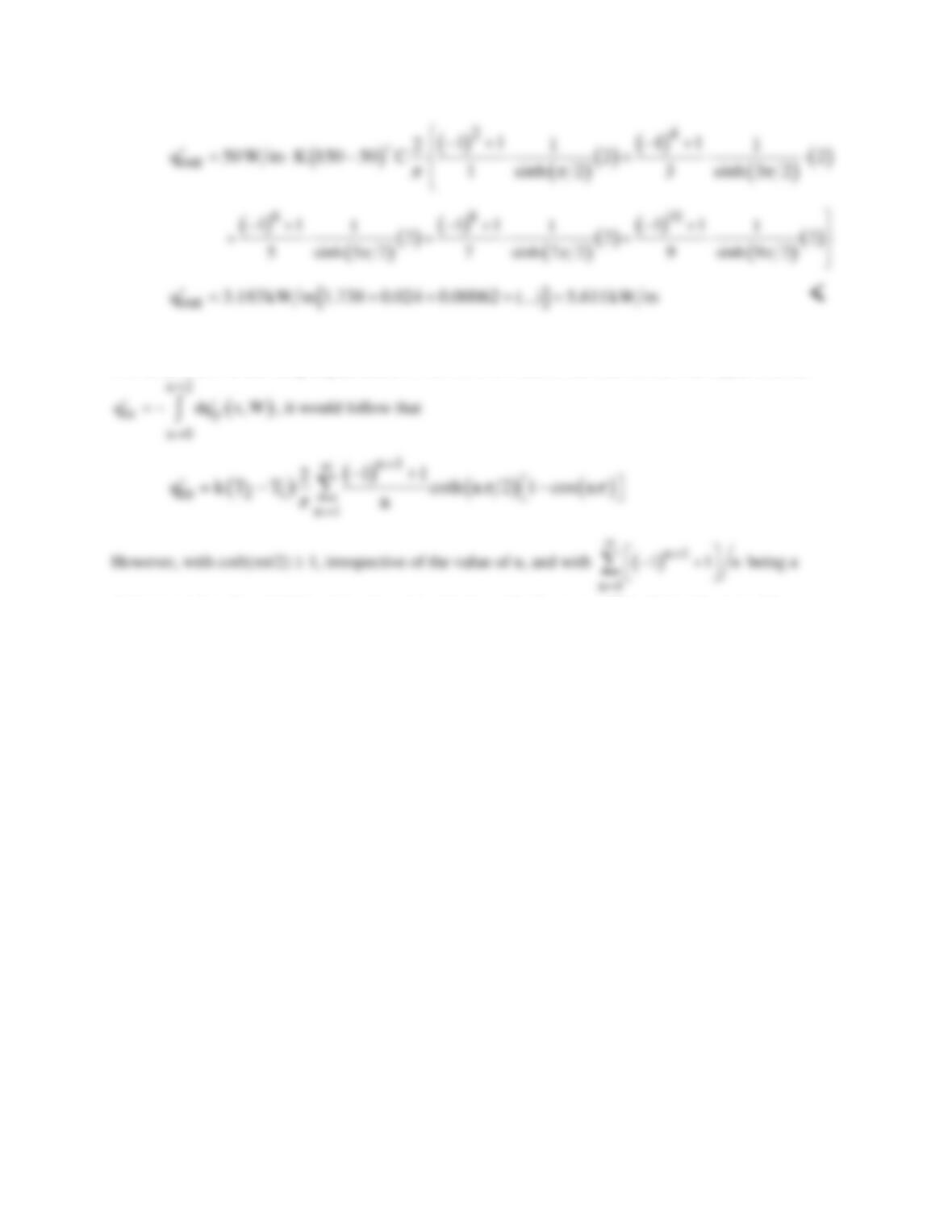
ANALYSIS: The heat rate per unit thickness from the plate along the lower surface is
where from the solution to Problem 4.2,
Evaluate the gradient of θ from Eq. (2) and substitute into Eq. (1) to obtain
n1
=
To evaluate the first five, non–zero terms, recognize that since cos(nπ) = 1 for n = 2, 4, 6 …, only the n-
odd terms will be non-zero. Hence,
Continued …
PROBLEM 4.3 (Cont.)
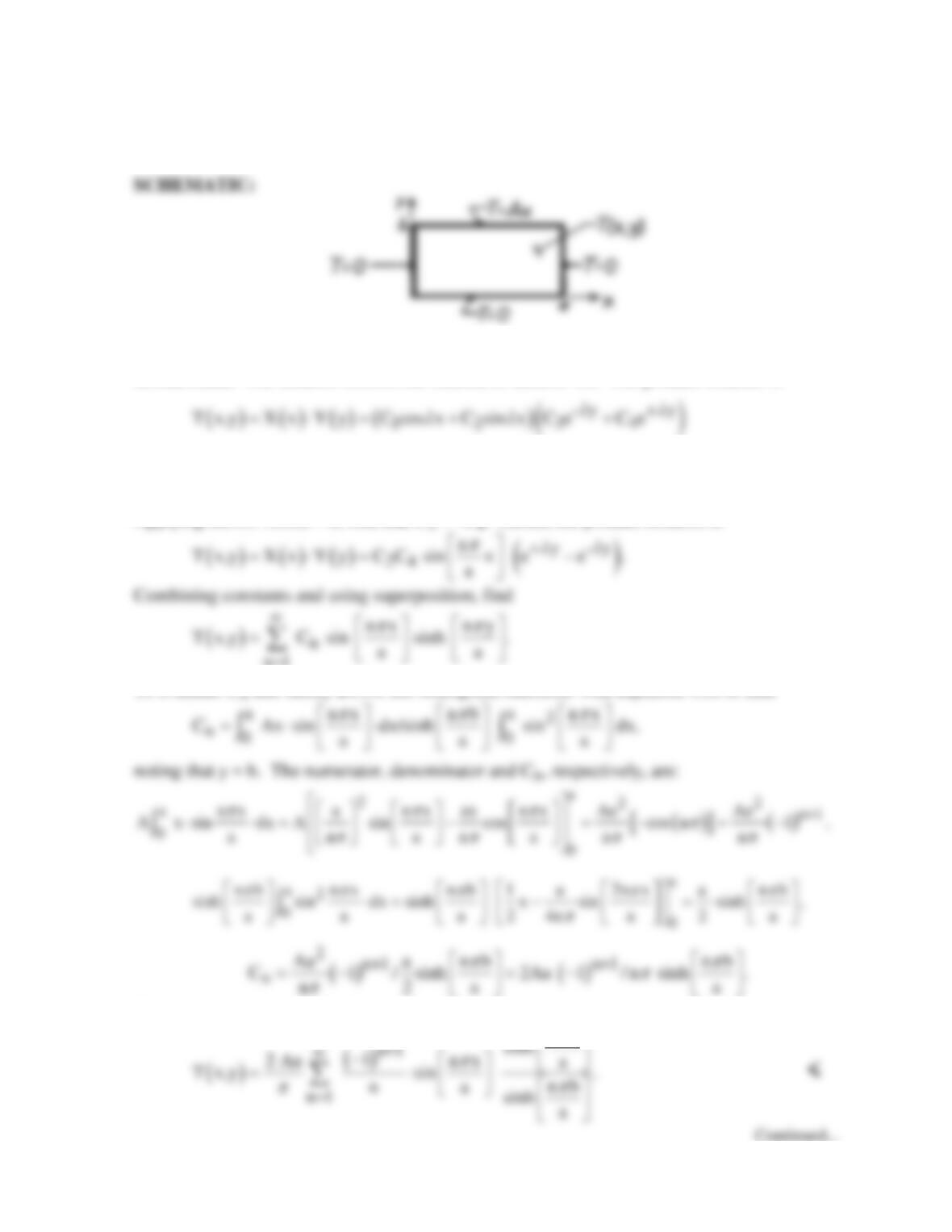
COMMENTS: If the foregoing procedure were used to evaluate the heat rate into the upper surface,
divergent series, the complete series does not converge and
in
q′→∞
. This physically untenable
condition results from the temperature discontinuities imposed at the upper left and right corners.
PROBLEM 4.4
KNOWN: Rectangular plate subjected to prescribed boundary conditions.
FIND: Steady–state temperature distribution and heat flux distribution along top edge.
ASSUMPTIONS: (1) Steady–state, 2-D conduction, (2) Constant properties.
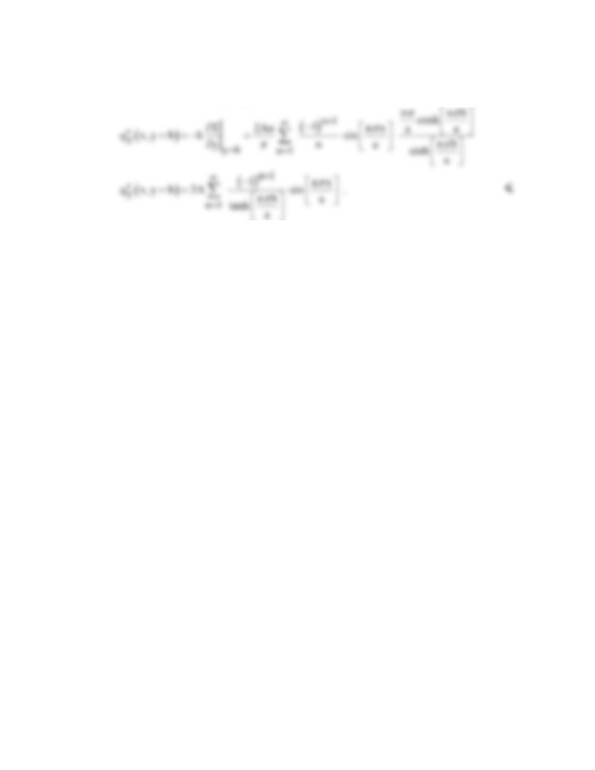
ANALYSIS: The solution follows the method of Section 4.2. The product solution is
and the boundary conditions are: T(0,y) = 0, T(a,y) = 0, T(x,0) = 0, T(x.b) = Ax. Applying
BC#1, T(0,y) = 0, find C1 = 0. Applying BC#2, T(a,y) = 0, find that λ = nπ/a with n = 1,2,….
Applying BC#3, T(x,0) = 0, find that C3 = -C4. Hence, the product solution is
n1
=
To evaluate Cn and satisfy BC#4, use orthogonal functions with Equation 4.16 to find
Hence, the temperature distribution is
ny
π
PROBLEM 4.4 (Cont.)
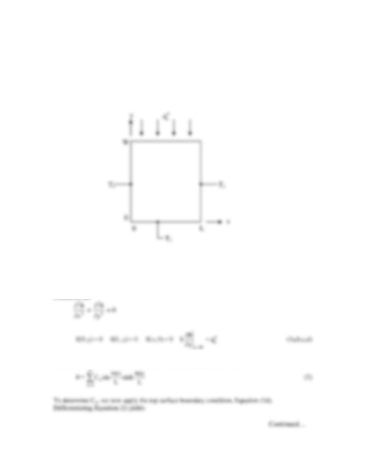
The heat flux normal to the top edge can be found from Fourier’s Law:
COMMENTS: The heat transfer rate out of the top edge can be found by integrating the heat
flux expression above over the x-direction. If this is done similarly for all four surfaces, and
the results summed, the net heat transfer rate leaving the rectangle must come out to zero
since it is at steady-state with no heat generation.
PROBLEM 4.5
KNOWN: Boundary conditions on four sides of a rectangular plate.
FIND: Temperature distribution.
SCHEMATIC:
ASSUMPTIONS: (1) Two–dimensional, steady-state conduction, (2) Constant properties.
ANALYSIS: This problem differs from the one solved in Section 4.2 only in the boundary
condition at the top surface. Defining θ = T – T∞, the differential equation and boundary
conditions are
The solution is identical to that in Section 4.2 through Equation (4.11),
PROBLEM 4.5 (Cont.)
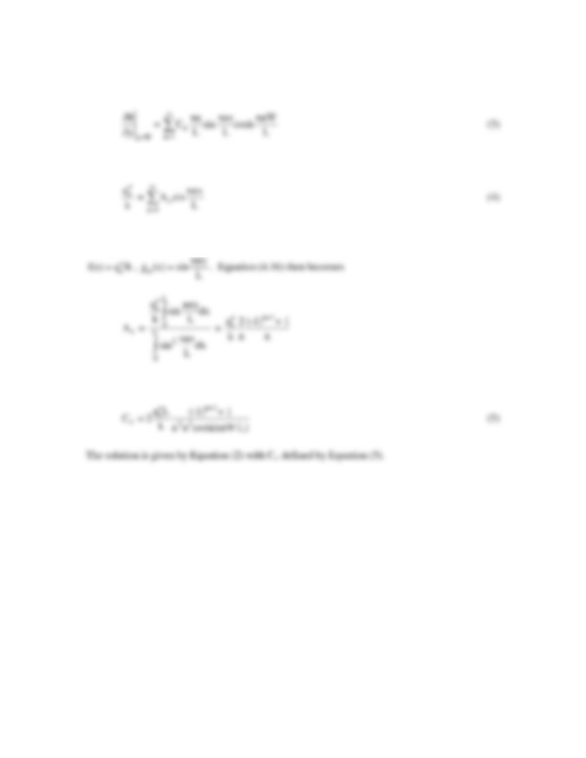
Substituting this into Equation (1d) results in
where An = Cn(nπ/L)cosh(nπW/L). The principles expressed in Equations (4.13) through (4.16)
still apply, but now with reference to Equation (4) and Equation (4.14), we should choose
Thus
PROBLEM 4.6
KNOWN: Diameters and temperatures of horizontal circular cylinders. Eccentricity factor. Heat
transfer rate per unit length. Fluid thermal conductivity.
FIND: Effective thermal conductivity.
ASSUMPTIONS: (1) Constant properties, (2) Steady state conditions.
PROPERTIES: Given: k = 0.255 W/m⋅K.
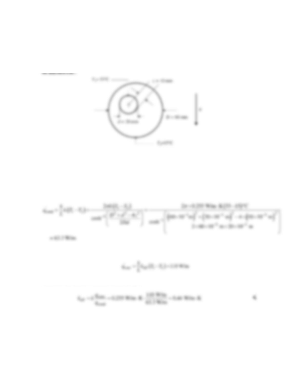
ANALYSIS: In the absence of free convection the conduction heat transfer per unit length may be found
by using the shape factor expression and applying Case 7 of Table 4.1. Hence
The free convection heat transfer rate is
Therefore the effective thermal conductivity is
COMMENTS: Buoyancy-induced fluid motion increases the heat transfer rate between the
cylinders by 74%.
PROBLEM 4.7
KNOWN: Boundary conditions on four sides of a square plate.
FIND: Expressions for shape factors associated with the maximum and average top surface
temperatures. Values of these shape factors. The maximum and average temperatures for
specified conditions.
SCHEMATIC:
ASSUMPTIONS: (1) Two–dimensional, steady-state conduction, (2) Constant properties.
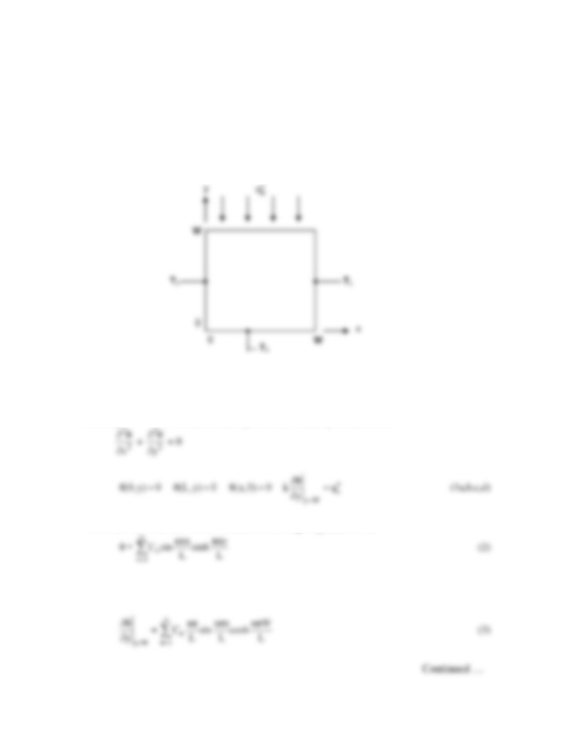
ANALYSIS: We must first find the temperature distribution as in Problem 4.5. Problem 4.5
differs from the problem solved in Section 4.2 only in the boundary condition at the top surface.
Defining θ = T – T∞, the differential equation and boundary conditions are
The solution is identical to that in Section 4.2 through Equation (4.11),
To determine Cn, we now apply the top surface boundary condition, Equation (1d).
Differentiating Equation (2) yields
PROBLEM 4.7 (Cont.)
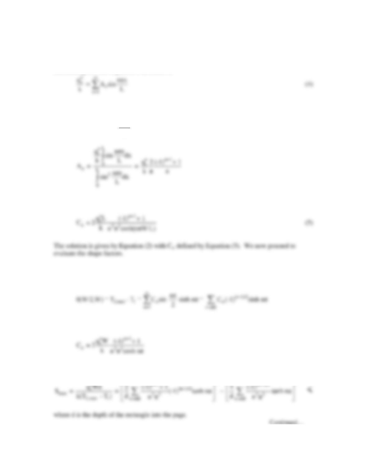
Substituting this into Equation (1d) results in
where An = Cn(nπ/L)cosh(nπW/L). The principles expressed in Equations (4.13) through (4.16)
still apply, but now with reference to Equation (4) and Equation (4.14), we should choose
s
f(x) = q /k
′′
,
n
nπx
g (x) = sin L
. Equation (4.16) then becomes
Thus
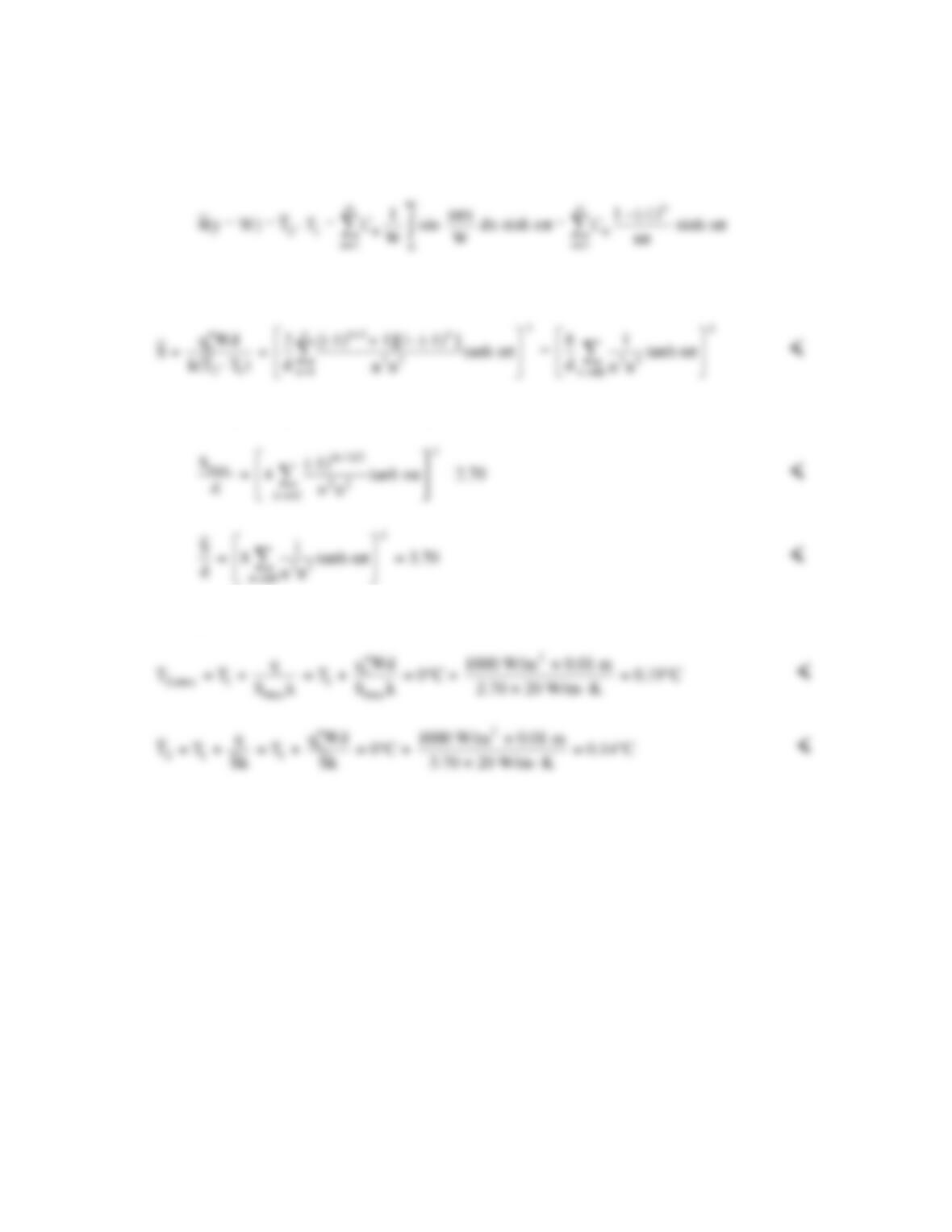
(a) The maximum top surface temperature occurs at the midpoint of that surface, x = W/2, y = W.
From Equation (2) with L = W,
where
Thus
-1 -1
PROBLEM 4.7 (Cont.)
(b) The average top surface temperature is given by
Thus
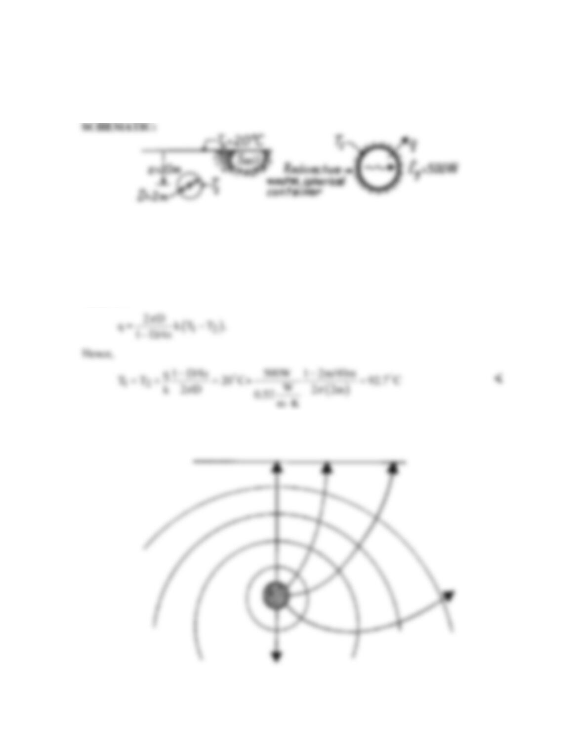
(c) Evaluating the expressions for the shape factors yields
The temperatures can then be found from
PROBLEM 4.8
KNOWN: Heat generation in a buried spherical container.
FIND: (a) Outer surface temperature of the container, (b) Representative isotherms and heat
flow lines.
ASSUMPTIONS: (1) Steady-state conditions, (2) Soil is a homogeneous medium with
constant properties.
PROPERTIES: Table A-3, Soil (300K): k = 0.52 W/m⋅K.
ANALYSIS: (a) From an energy balance on the container,
g
qE=
and from the first entry in
Table 4.1,
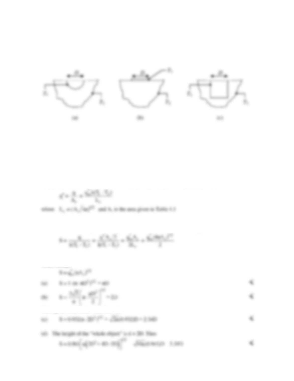
(b) The isotherms may be viewed as spherical surfaces whose center moves downward with
increasing radius. The surface of the soil is an isotherm for which the center is at z = ∞.
PROBLEM 4.9
KNOWN: Shape of objects at surface of semi-infinite medium.
FIND: Shape factors between object at temperature T1 and semi–infinite medium at temperature T2.
SCHEMATIC:
ASSUMPTIONS: (1) Steady-state, (2) Medium is semi-infinite, (3) Constant properties, (4) Surface
of semi–infinite medium is adiabatic.
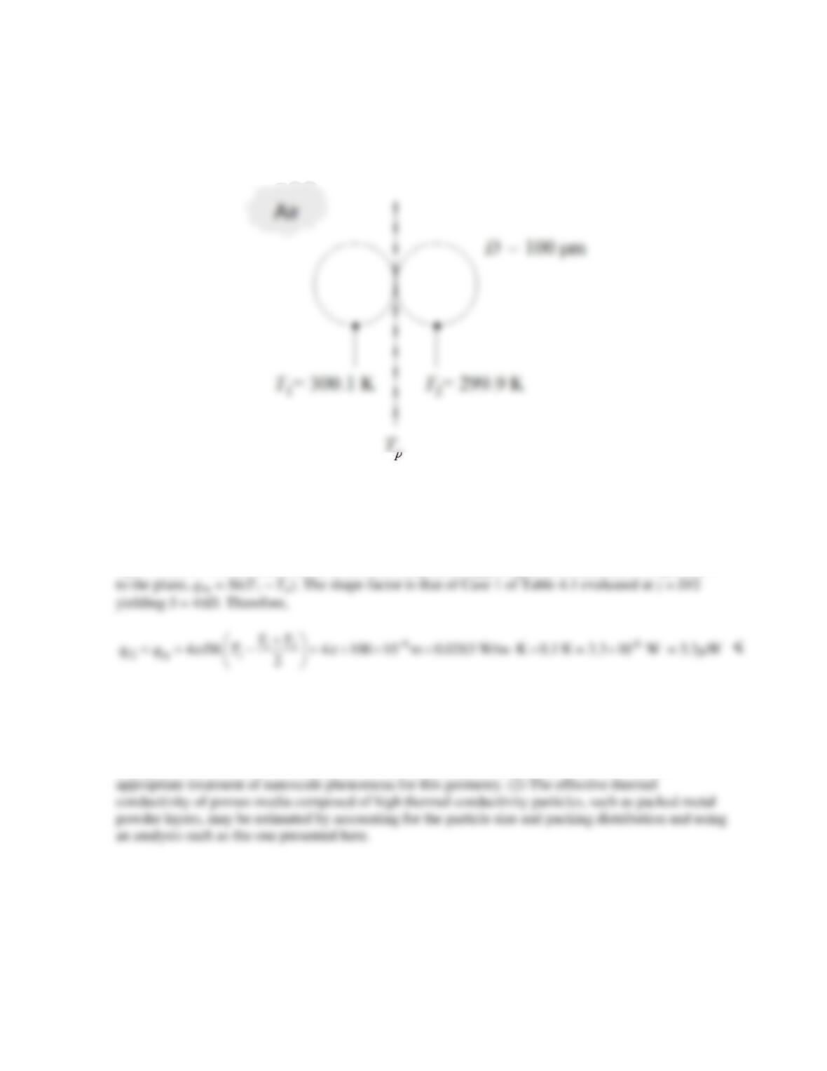
ANALYSIS: Cases 12 -15 of Table 4.1 all pertain to objects buried in an infinite medium. Since
they all possess symmetry about a horizontal plane that bisects the object, they are equivalent to the
cases given in this problem for which the horizontal plane is adiabatic. In particular, the heat flux is
the same for the cases of this problem as for the cases of Table 4.1. Note, that when we use Table 4.1
to determine the dimensionless conduction heat rate,
*
ss
q
, we must be consistent and use the surface
area of the “entire” object of Table 4.1, not the “half” object of this problem. Then
When we calculate the shape factors we must account for the fact that the surface areas and heat
transfer rates for the objects of this problem are half as much as for the objects of Table 4.1.
where As is still the area in table 4.1 and the 2 in the denominator accounts for the area being halved.
Thus, finally,
This agrees with Table 4.1a, Case 10.
PROBLEM 4.10
KNOWN: Diameters and temperatures of spherical particles that are in contact.
FIND: Heat transfer rate.
SCHEMATIC:
ASSUMPTIONS: (1) Constant properties, (2) Isothermal particles.
PROPERTIES: Table A.4, Air (300 K): k = 0.0263 W/m⋅K.
ANALYSIS: By symmetry, the vertical plane at the particle contact point is at temperature Tp = (T1 +
T2)/2 = 300 K. Therefore, conduction between the particles q12 is equal to conduction from particle 1
COMMENTS: (1) The air thermal conductivity in the vicinity of the contact point would be
reduced by nanoscale effects such as those described in Chapter 2. In applying the shape factor of
Case 1 of Table 4.1 to the z = D/2 situation we have implicitly assumed that nanoscale effects are
negligible. See B. Gebhart, Heat Conduction and Mass Diffusion, McGraw–Hill, 1993 for an
PROBLEM 4.11
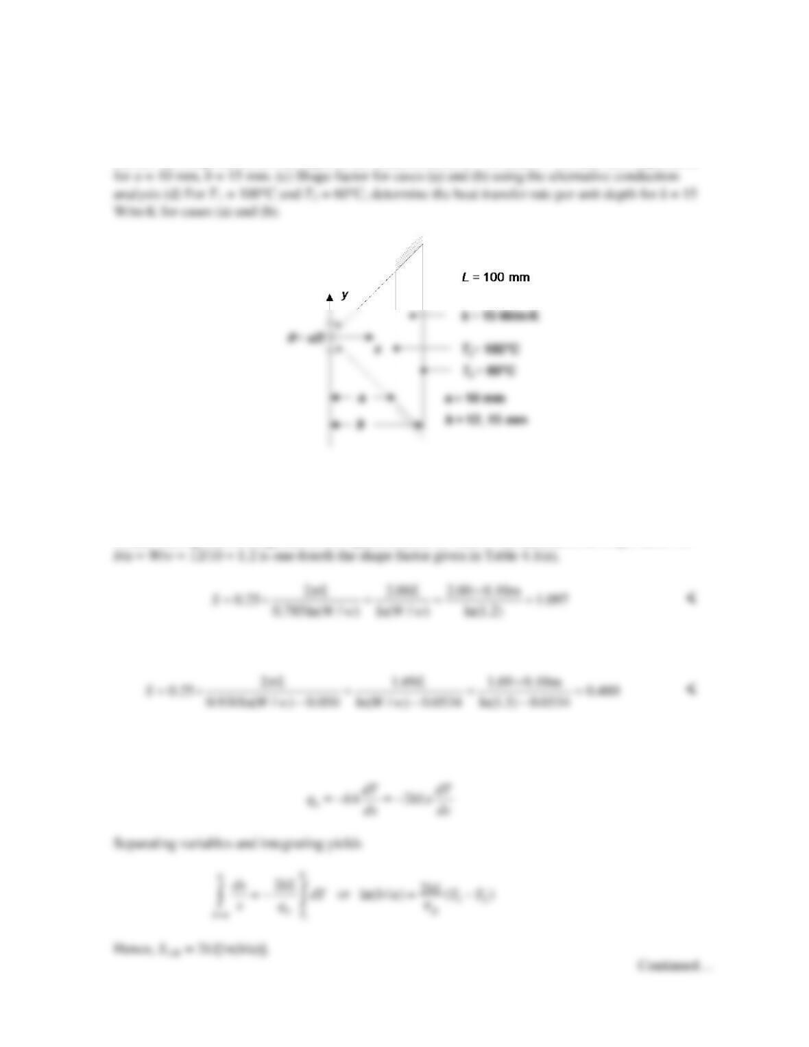
KNOWN: Dimensions of a two–dimensional object, applied boundary conditions and thermal
conductivity.
FIND: (a) Shape factor for the object if the dimensions are a = 10 mm, b = 12 mm. (b) Shape factor
SCHEMATIC:
ASSUMPTIONS: (1) Steady–state conditions, (2) Constant properties.
PROPERTIES: Given: k = 15 W/m⋅K.
ANALYSIS: (a) The geometry and applied boundary conditions correspond to Case 11 of Table
4.1(a). Noting that the diagonals of the square channel of Case 11 are adiabats, the shape factor for
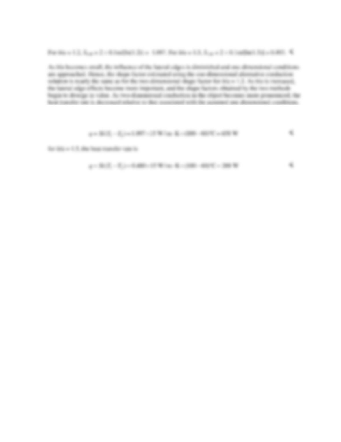
(b) For b/a = W/w = 15/10 = 1.5,
(c) From the one-dimensional alternative conduction analysis with the top surface described by y = x
and A = 2yL,
PROBLEM 4.11 (Cont.)
(d) For b/a = 1.2, the heat transfer rate is
COMMENTS: The heat transfer rate is independent of the individual values of a or b. As either b or
a is increased while maintaining a fixed b/a ratio, the cross-sectional area for heat transfer increases,
but the increase is offset by increased thickness through which the conduction occurs. The offsetting
effects balance one another, and the net result is no change in the heat transfer rate.
PROBLEM 4.12
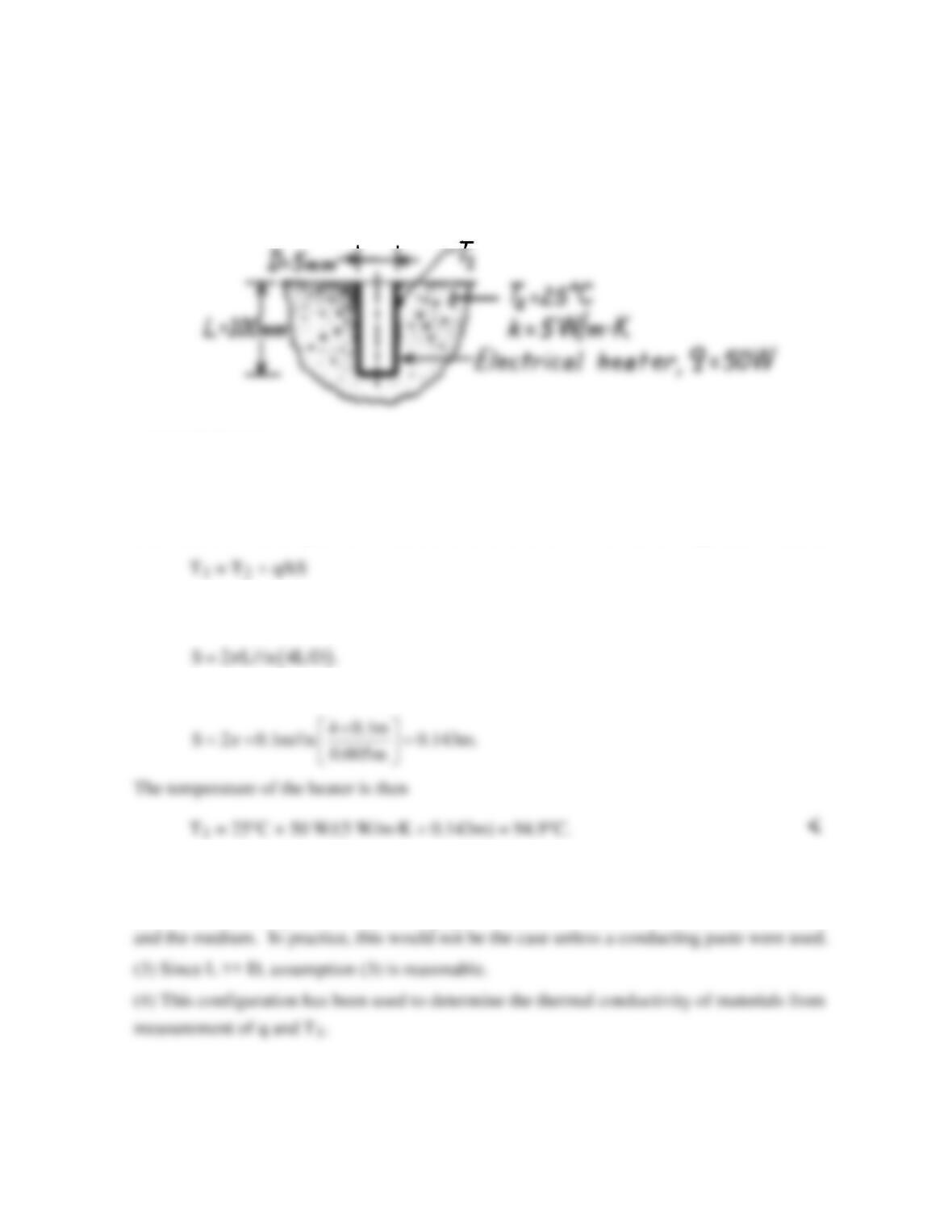
KNOWN: Electrical heater of cylindrical shape inserted into a hole drilled normal to the
surface of a large block of material with prescribed thermal conductivity.
FIND: Temperature reached when heater dissipates 50 W with the block at 25°C.
SCHEMATIC:
ASSUMPTIONS: (1) Steady-state conditions, (2) Block approximates semi-infinite medium
with constant properties, (3) Negligible heat loss to surroundings above block surface, (4)
Heater can be approximated as isothermal at T1.
ANALYSIS: The temperature of the heater surface follows from the rate equation written as
where S can be estimated from the conduction shape factor given in Table 4.1 for a “vertical
cylinder in a semi–infinite medium,”
Substituting numerical values, find
COMMENTS: (1) Note that the heater has L >> D, which is a requirement of the shape
factor expression.
(2) Our calculation presumes there is negligible thermal contact resistance between the heater
PROBLEM 4.13
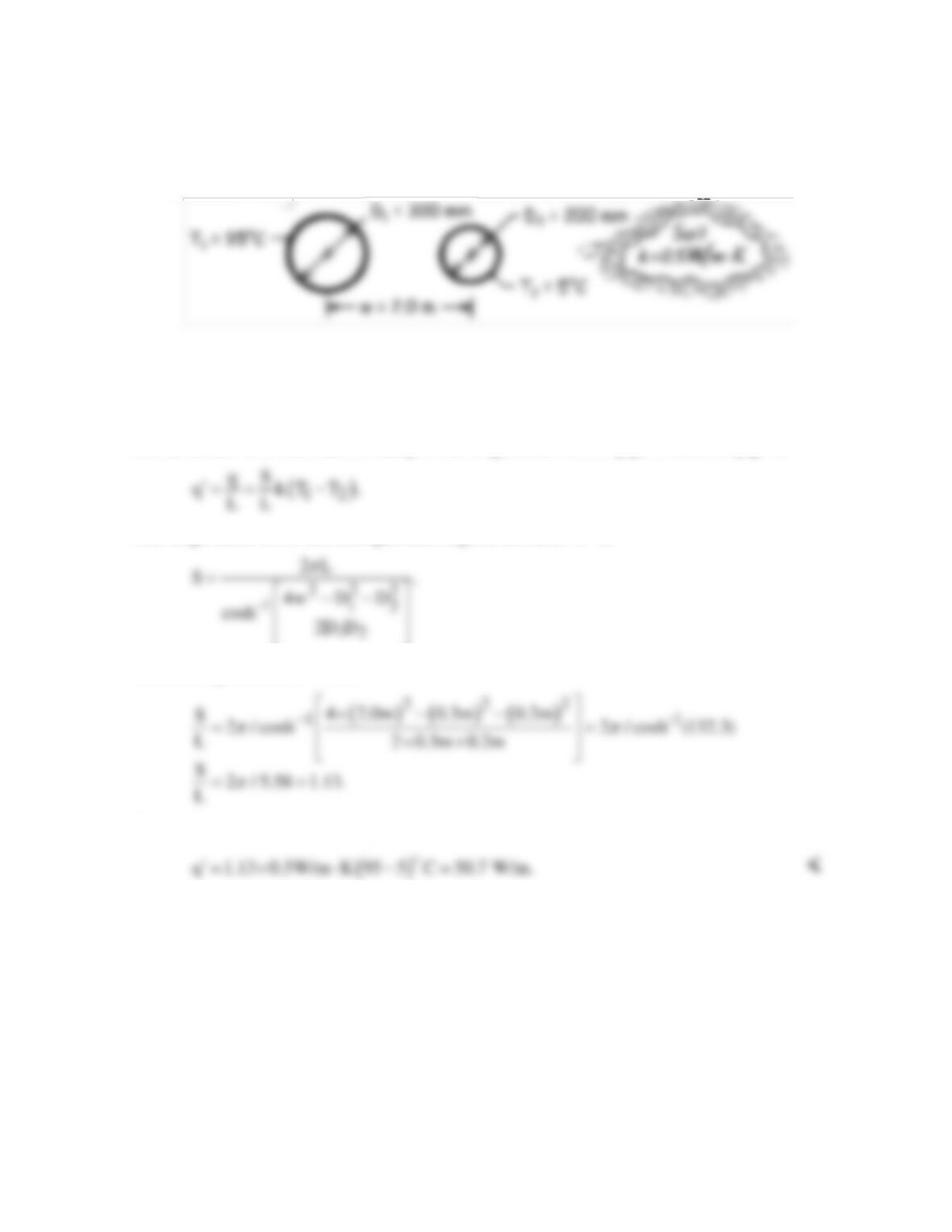
KNOWN: Surface temperatures of two parallel pipe lines buried in soil.
FIND: Heat transfer per unit length between the pipe lines.
SCHEMATIC:
ASSUMPTIONS: (1) Steady-state conditions, (2) Two-dimensional conduction, (3)
Constant properties, (4) Pipe lines are buried very deeply, approximating burial in an infinite
medium, (5) Pipe length >> D1 or D2 and w > D1 or D2.
ANALYSIS: The heat transfer rate per unit length from the hot pipe to the cool pipe is
The shape factor S for this configuration is given in Table 4.1 as
Substituting numerical values,
Hence, the heat rate per unit length is
COMMENTS: The heat gain to the cooler pipe line will be larger than 50.7 W/m if the soil
temperature is greater than 5°C. How would you estimate the heat gain if the soil were at
25°C?