Section 6.3: Applications Involving Powers of Matrices 375
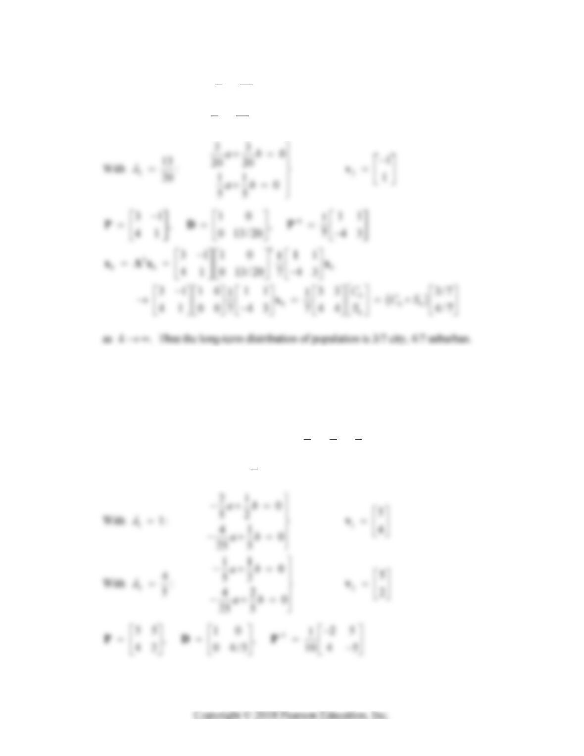
With
11:
13 0
520
13 0
520
ab
ab
1
3
4
v
In the following three problems, just as in Problems 25–30, we first write the elements of A in
fractional rather than decimal form, with r = 4/25 in Problem 31, r = 7/40 in Problem 32, and
r = 27/200 in Problem 33.
31. Characteristic polynomial: 2941
() ( 1)(5 4)
555
p
Eigenvalues: 12
4
1, 5
376 Chapter 6: Eigenvalues and Eigenvectors
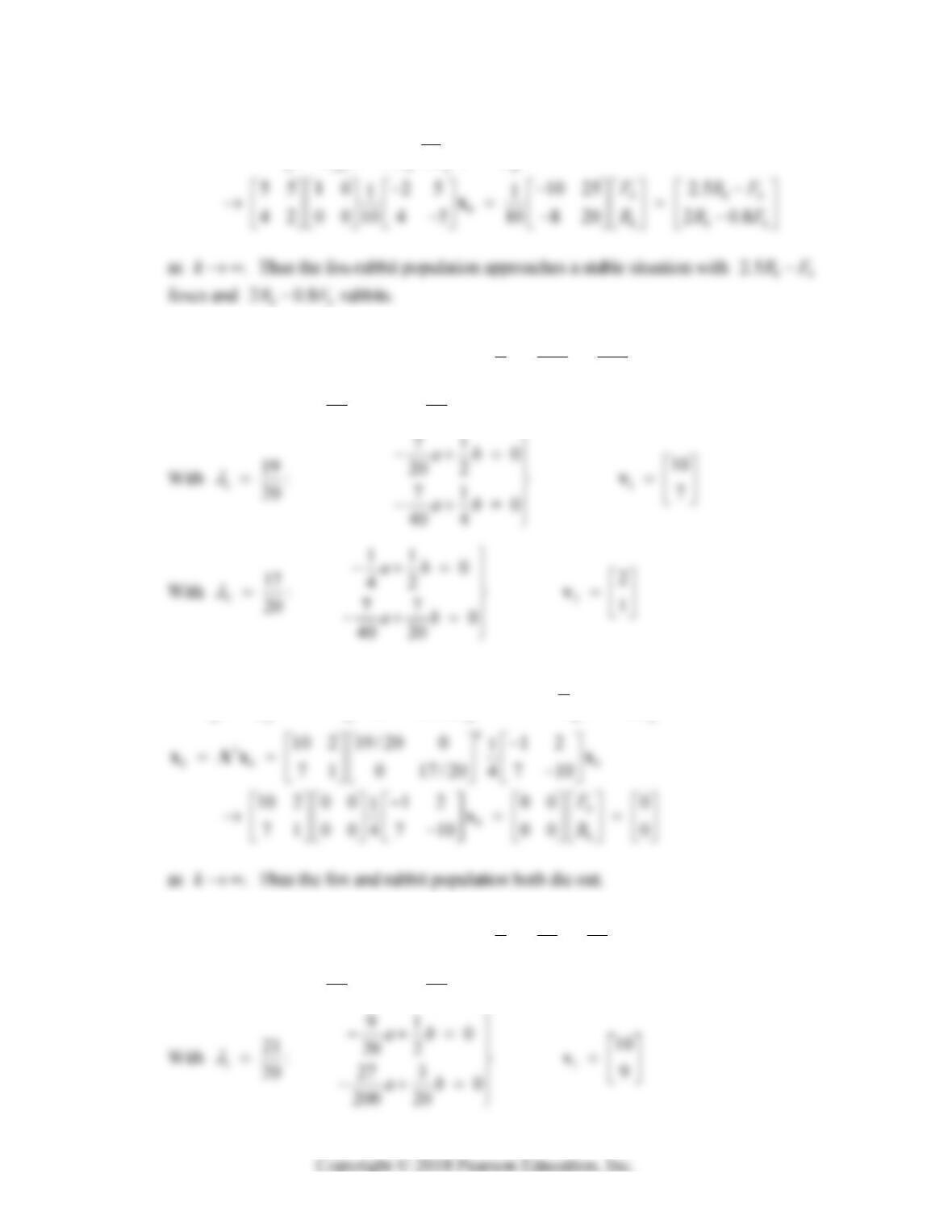
00
551 0 2 5
1
4204/5 4 5
10
k
k
k
xAx x
32. Characteristic polynomial: 29 323 1
( ) (20 19)(20 17)
5 400 400
p
Eigenvalues: 12
19 17
,
20 20
1
10 2 19 / 20 0 1 2
1
,,
71 0 17/20 7 10
4
PD P
33. Characteristic polynomial: 2963 1
( ) (20 21)(4 3)
58080
p
Eigenvalues: 12
19 17
,
20 20
Section 6.3: Applications Involving Powers of Matrices 377
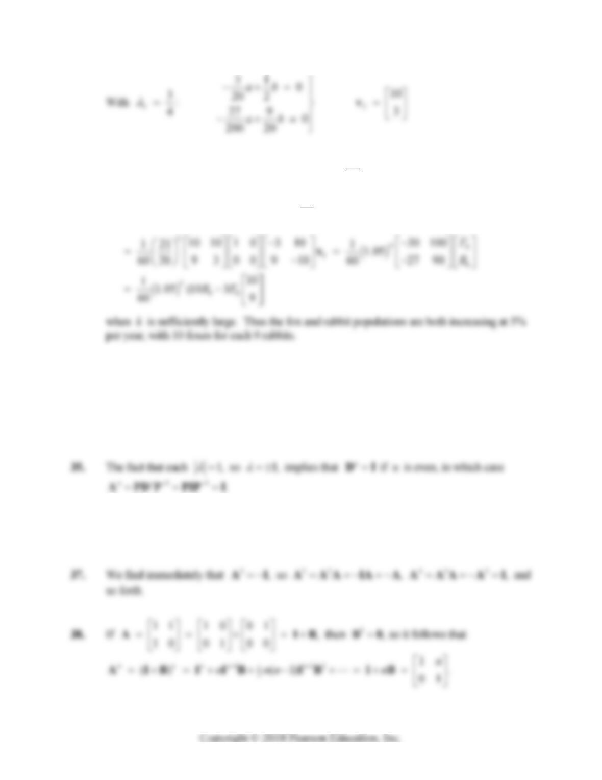
1
00
10 10 21/ 20 0 3 10
1
,,
93 0 3/4 9 10
60
10 10 21/ 20 0 3 10
1
93 0 3/4 9 10
60
k
k
k
PD P
xAx x
34. 13 5 1 0 7 5 41 30
4 7 0 1 4 3 56 41
APDP
If n is even then nDI so 11
.
nn
APDP PIP I
If n is odd then
1.
nn
AAAIAA Thus 99 100
and .AA A I
36. We find immediately that 232 432
,so , ,A I A AAIAAA AAA I and so
forth.
378 Chapter 6: Eigenvalues and Eigenvectors
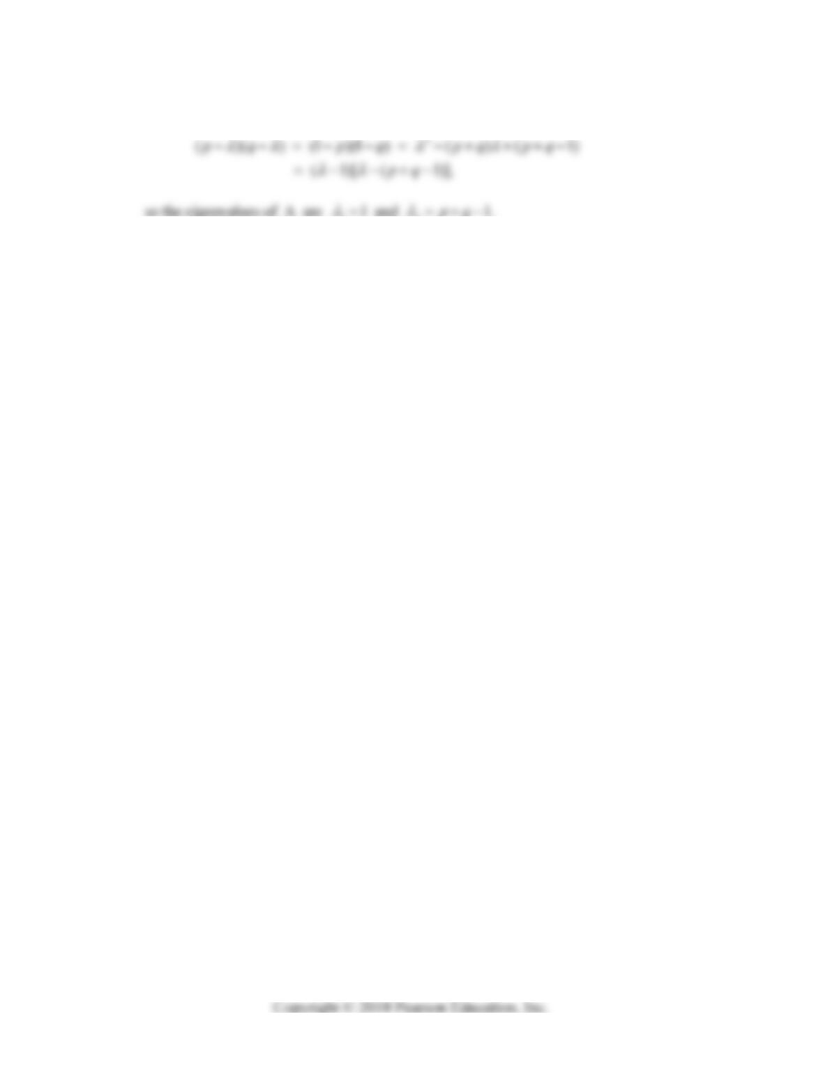
39. The characteristic equation of A is
40. The fact that the column sums of A are each 1 implies that the row sums of the transpose
matrix AT are each 1, so it follows readily that ATv = v. Thus 1
is an eigenvalue of
AT. But A and AT have the same eigenvalues (by Problem 35 in Section 6.1).
379
CHAPTER 7
LINEAR SYSTEMS OF
DIFFERENTIAL EQUATIONS
SECTION 7.1
FIRST-ORDER SYSTEMS AND APPLICATIONS
1. Let 2
1212
and , so 7 3 .
x
xxxxxxxxt
x
x
2. Let
121 32 43
,, , ,soxxxxxxxxxxx
(4)
436 cos3.
x
xxxx t
Equivalent system:
1
x
= x2, 2
x
= x3, 3
x
= x4, 4
x
= –x1 + 3x2 – 6x3 + cos 3t
x
x
x
5. Let
2
121 32 3
,, ,so cos.
x
xx x x x x x x x x x
Equivalent system:
1
x
= x2, 2
x
= x3, 3
x
= x2
2 + cos x1
x
380 Chapter 7: Linear Systems of Differential Equations
7. Let 223/2
121 1 21 2
,,, so /(),xxxxxyyyyy xx kxxy
223/2
2/( ) .yy kyxy
y
y
8. Let
121 1 21 2
,,, so423,
x
xx x x y yy y y x x x y x
232cos.
y
yxyy t
Equivalent system:
x
x
y
y
9. Let
121 1 21 121
,,, ,,,soxxxxxyyy yyzzzzz
232,
x
xxyz
22
4, 5 .
y
yxy zz z xyz
Equivalent system:
x
x
y
y
10. Let
121 1 21 2
,,, so(1),
x
xxxxyyyyy xxx y
2(1 ).
y
yy x
Equivalent system:
x
x
y
y
11. The computation x” = y’ = –x yields the single linear second-order equation
x” + x = 0 with characteristic equation r2 + 1 = 0 and general solution
x(t) = A cos t + B sin t.
Section 7.1: First-Order Systems and Applications 381
Then the original first equation y = x’ gives
y(t) = B cos t – A sin t.
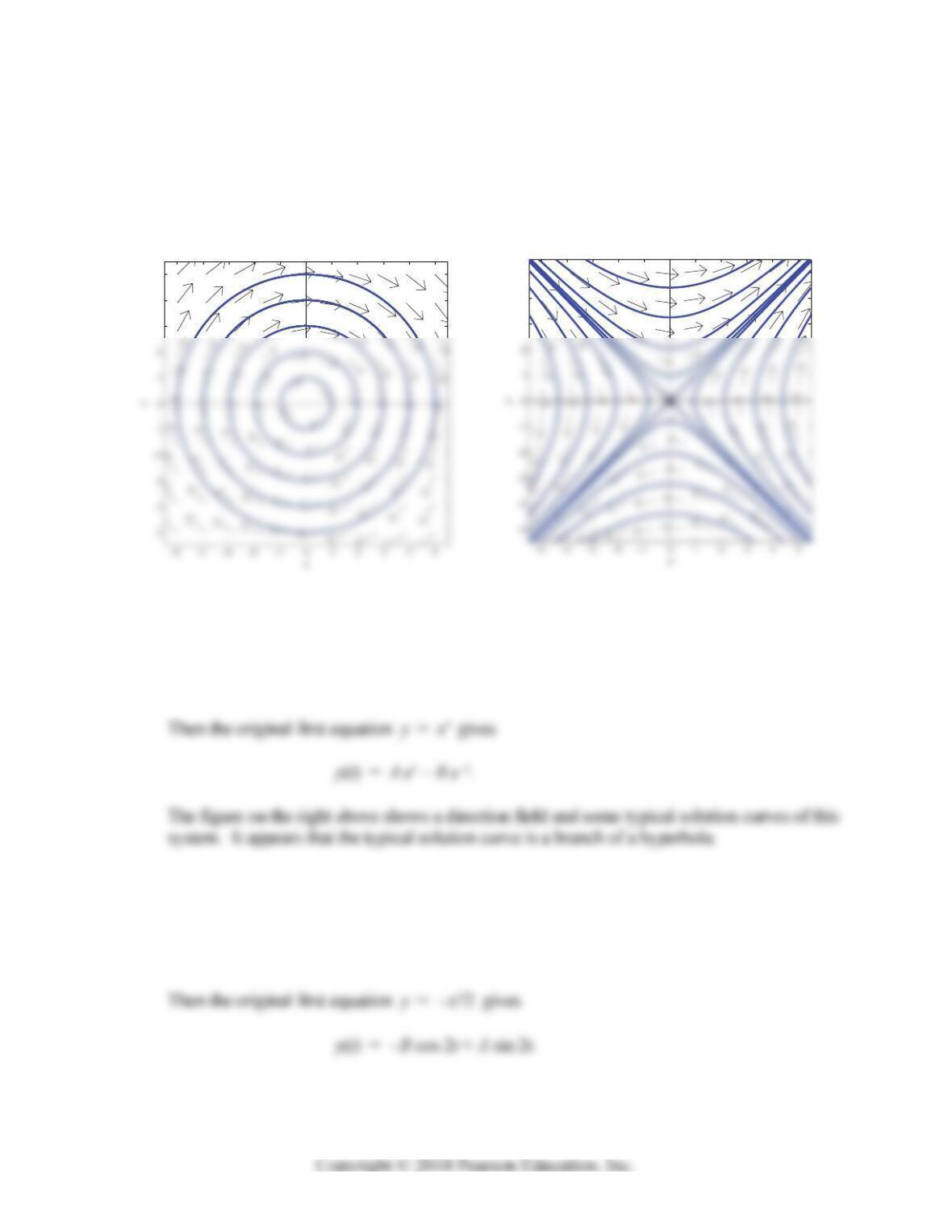
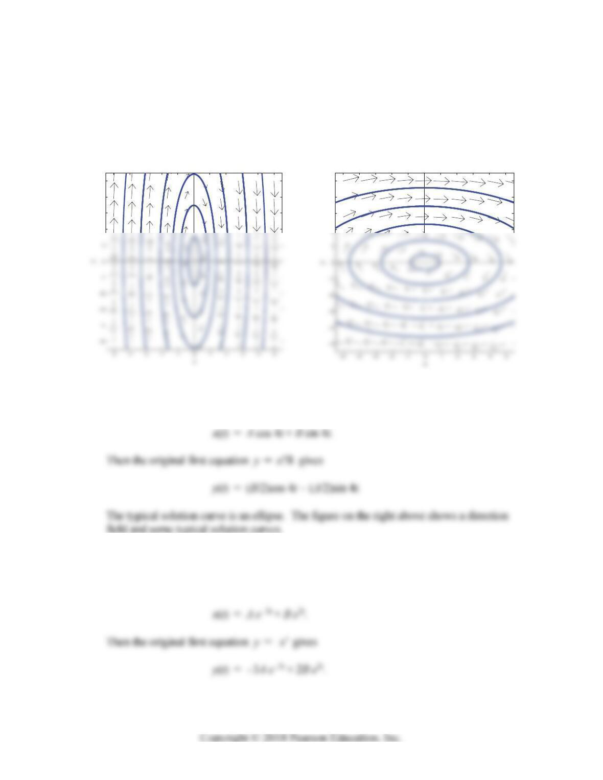
The figure on the left below shows a direction field and typical solution curves (obviously
circles?) for the given system.
12. The computation x” = y’ = x yields the single linear second-order equation
x” – x = 0 with characteristic equation r2 – 1 = 0 and general solution
x(t) = A et + B e–
t.
13. The computation x” = –2y’ = –4x yields the single linear second-order equation
x” + 4x = 0 with characteristic equation r2 + 4 = 0 and general solution
x(t) = A cos 2t + B sin 2t.
3
4
5
3
4
5
382 Chapter 7: Linear Systems of Differential Equations
14. The computation x” = 10y’ = –100x yields the single linear second-order equation
x” + 100x = 0 with characteristic equation r2 + 100 = 0 and general solution
x(t) = A cos 10t + B sin 10t.
15. The computation x” = y’/2 = –4x yields the single linear second-order equation
x” + 4x = 0 with characteristic equation r2 + 4 = 0 and general solution
x(t) = A cos 2t + B sin 2t.
2
3
4
5
x
2
3
4
5
x
Section 7.1: First-Order Systems and Applications 383
2
3
4
5
Then the original first equation y = 2x’ gives
y(t) = 4B cos 2t – 4A sin 2t.
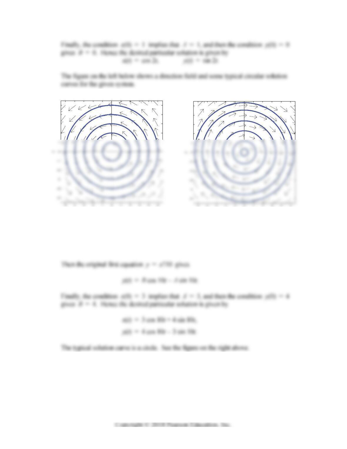
The figure on the left below shows a direction field and some typical elliptical
solution curves.
16. The computation x” = 8y’ = –16x yields the single linear second-order equation
x” + 16x = 0 with characteristic equation r2 + 16 = 0 and general solution
17. The computation x” = y’ = 6 x – y = 6 x – x’ yields the single linear second-order
equation x” + x’ – 6 x = 0 with characteristic equation r2 + r – 6 = 0 and characteristic
roots r = –3 and 2, so the general solution
2
3
4
5
384 Chapter 7: Linear Systems of Differential Equations
3
4
5
x
Finally, the initial conditions
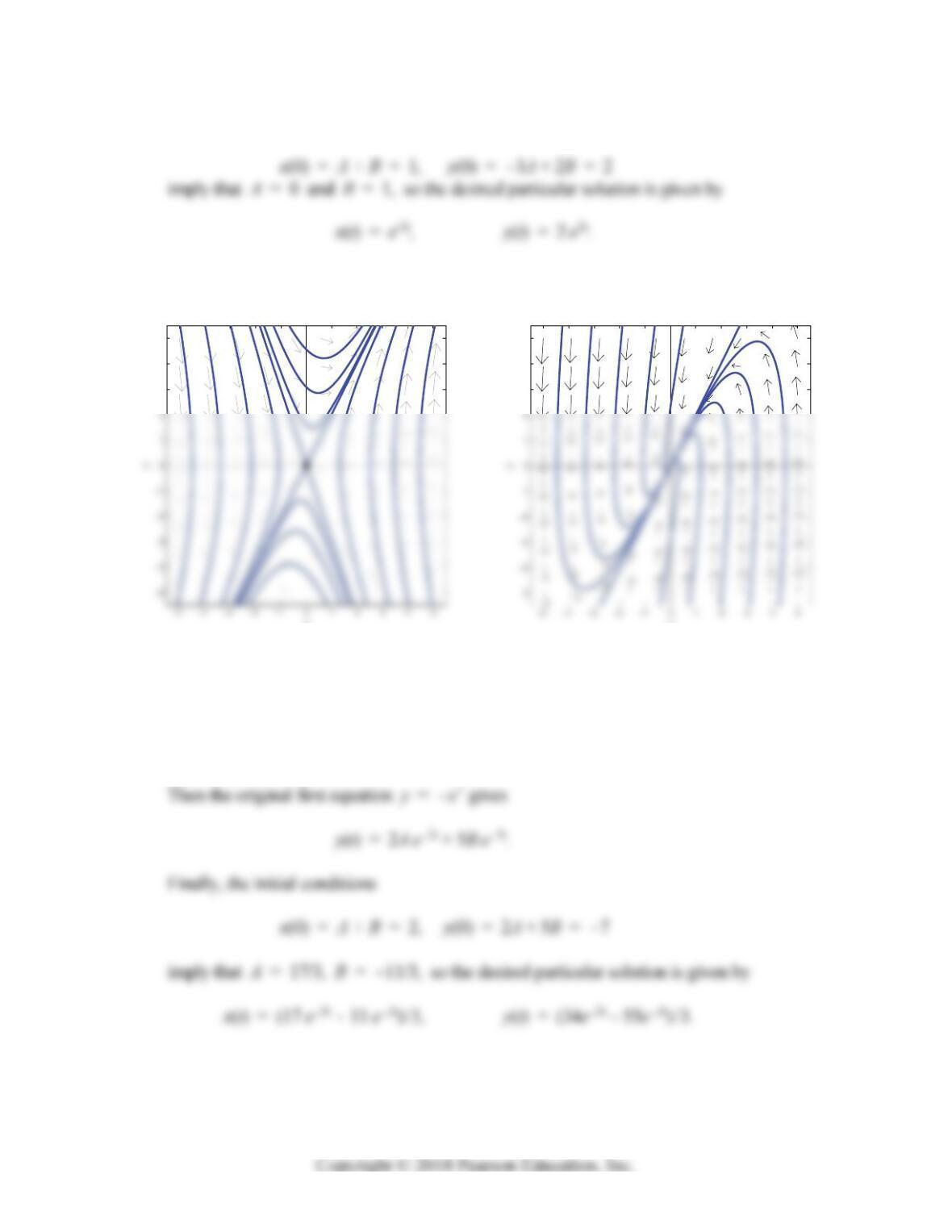
The figure on the left below shows a direction field and some typical solution curves.
18. The computation x” = –y’ = –10x + 7y = –10x – 7x’ yields the single linear second-
order equation x” + 7x’ + 10x = 0 with characteristic equation r2 + 7r + 10 = 0,
characteristic roots r = –2 and –5, and general solution
x(t) = A e–2t + B e–5t.
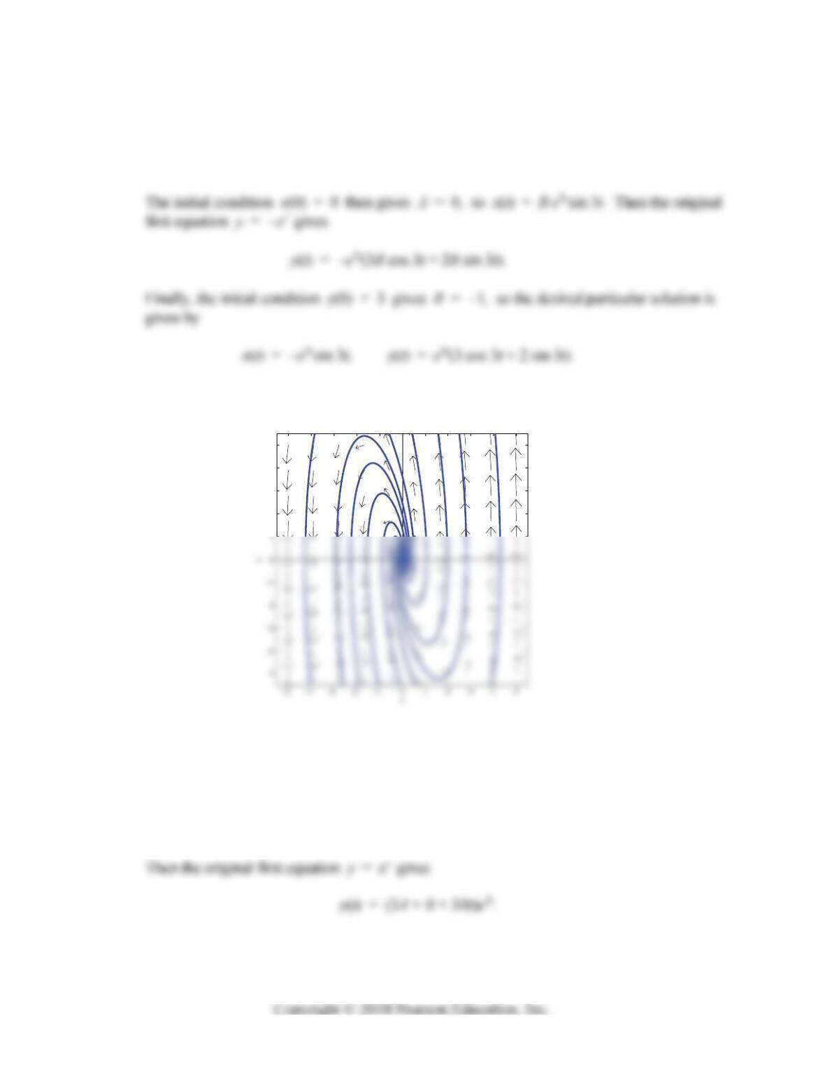
It appears that the typical solution curve is tangent to the straight line 2.
y
x See the
right-hand figure above for a direction field and typical solution curves.
3
4
5
x
Section 7.1: First-Order Systems and Applications 385
19. The computation x” = –y’ = –13x – 4y = –13x + 4x’ yields the single linear second-
order equation x” – 4x’ + 13x = 0 with characteristic equation r2 – 4r + 13 = 0 and
characteristic roots r = 2 ± 3i, hence the general solution is
x(t) = e2t(A cos 3t + B sin 3t).
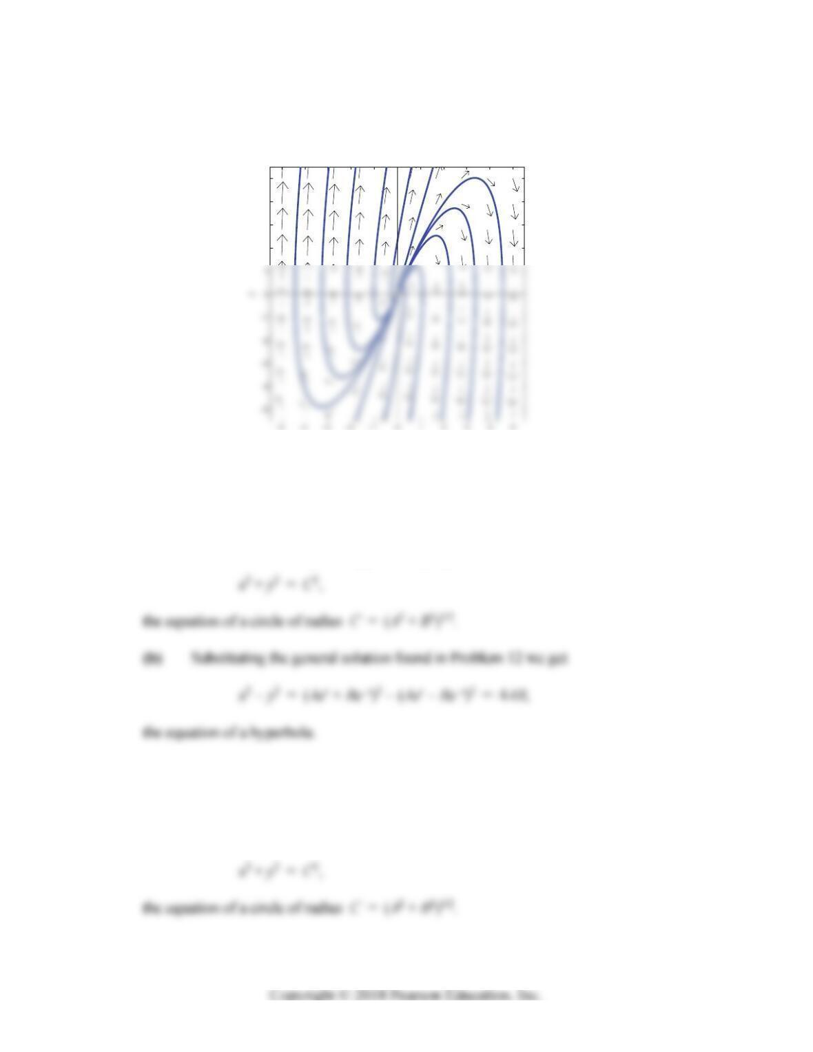
The figure below shows a direction field and some typical solution curves.
2
3
4
5
20. The computation x” = y’ = –9x + 6y = –9x + 6x’ yields the single linear second-order
equation x” – 6 x’ + 9 x = 0 with characteristic equation r2 – 6 r + 9 = 0 and repeated
characteristic root r = 3, 3, so its general solution is given by
x(t) = (A + Bt)e3t.
386 Chapter 7: Linear Systems of Differential Equations
It appears that the typical solution curve is tangent to the straight line 3 .
y
x The figure
at the top of the next page shows a direction field and some typical solution curves.
2
3
4
5
x
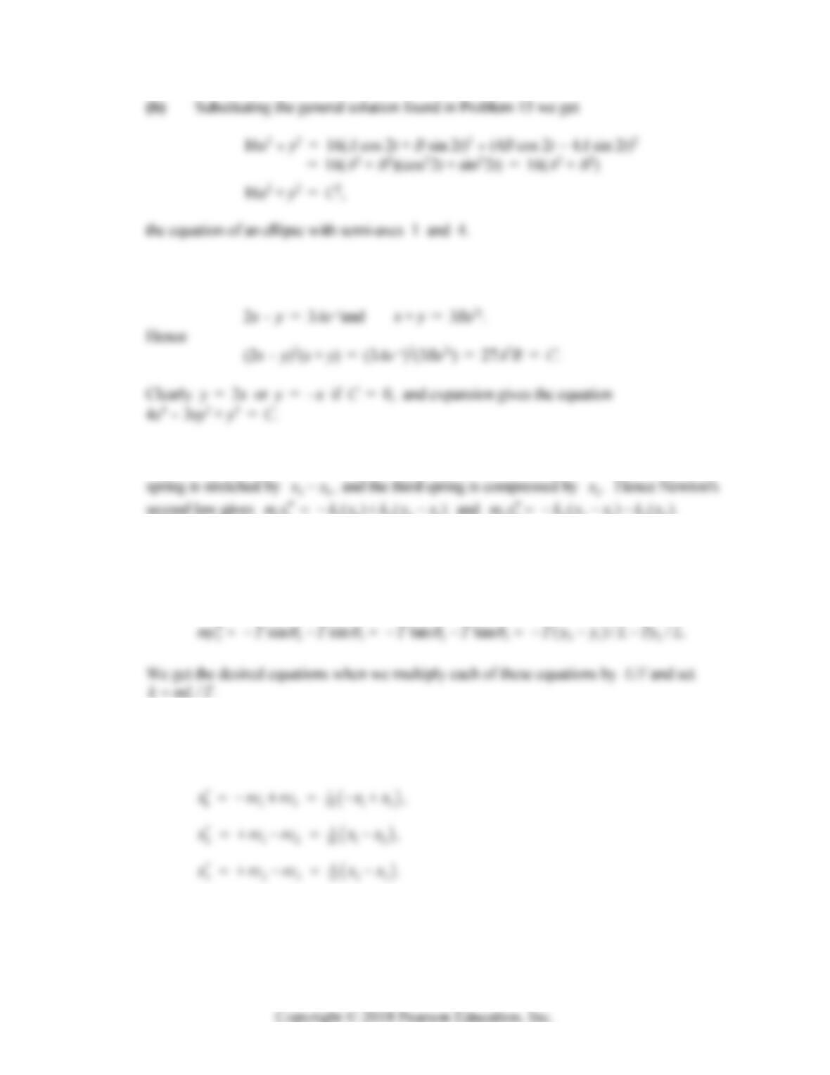
21. (a) Substituting the general solution found in Problem 11 we get
x2 + y2 = (Acos t + Bsin t)2 + (Bcos t – Asin t)2
= (A2 + B2)(cos2t + sin2t) = A2 + B2
22. (a) Substituting the general solution found in Problem 13 we get
x2 + y2 = (A cos 2t + B sin 2t)2 + (–B cos 2t + A sin 2t)2
= (A2 + B2)(cos22t + sin22t) = A2 + B2
Section 7.1: First-Order Systems and Applications 387
23. When we solve Equations (20) and (21) in the text for e–
t and e2t we get
24. Looking at Fig. 7.1.9 in the text, we see that the first spring is stretched by 1,
x
the second
25. Looking at Fig. 7.1.10 in the text, we see that
112 12121
sin sin tan tan / ( ) /my T T T T Ty L T y y L
,
26. The concentration of salt in tank i is /100
ii
cx for i = 1, 2, 3 and each inflow-outflow
rate is r = 10. Hence
x
27. If
is the polar angular coordinate of the point
,
x
y and we write
22 2
//,Fkx y kr then Newton’s second law gives
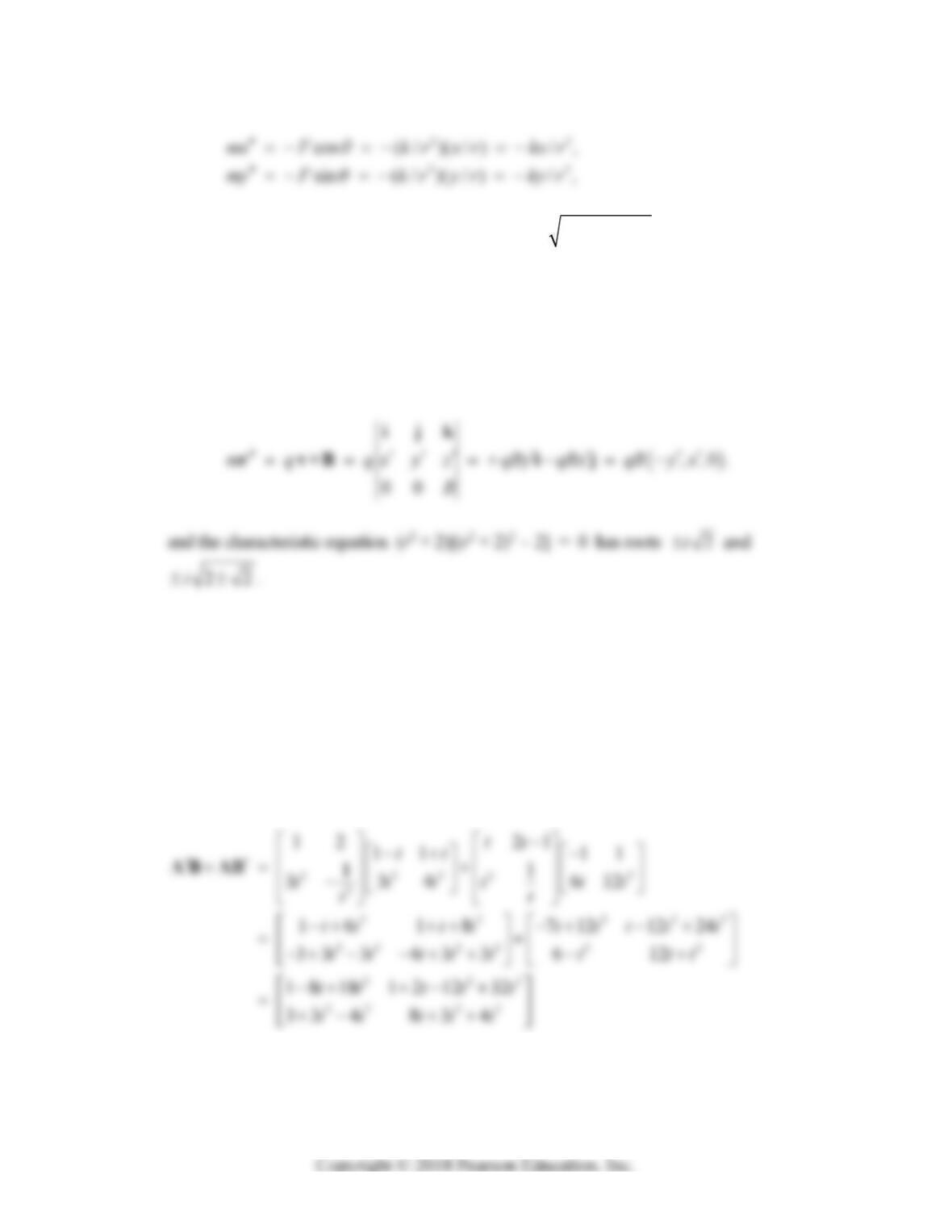
388 Chapter 7: Linear Systems of Differential Equations
28. If we write (x’, y’) for the velocity vector and
22
vxy
for the speed, then
(x’/v, y’/v) is a unit vector pointing in the direction of the velocity vector, and so the
components of the air resistance force Fr are given by
Fr = –kv2(x’/v, y’/v) = (–kvx’, –kvy’).
29. If ( , , )
x
yzr is the particle’s position vector, then Newton’s law m rF gives
SECTION 7.2
MATRICES AND LINEAR SYSTEMS
1.
23 234 2 2 3
34 234 2 3 2 3
4 6 4 8 1 8 18 1 2 12 32
() 34 334834
tt ttt t t t t t t t
tt t t t t t t t t t
AB
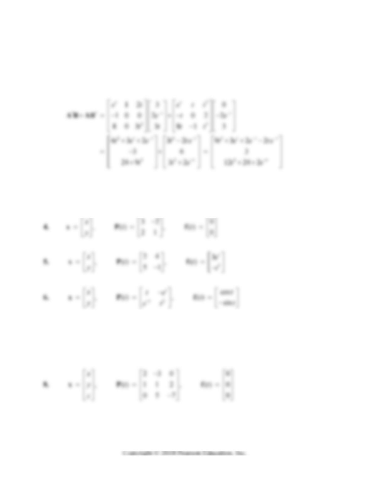
Section 7.2: Matrices and Linear Systems 389
2.
32
43
332 932 2
() 3 3
3 24 2 12 24 2
tt ttt
tt
tete tee te
t
tte t e
AB
3. 03 0
,() ,()
30 0
xtt
y
xP f
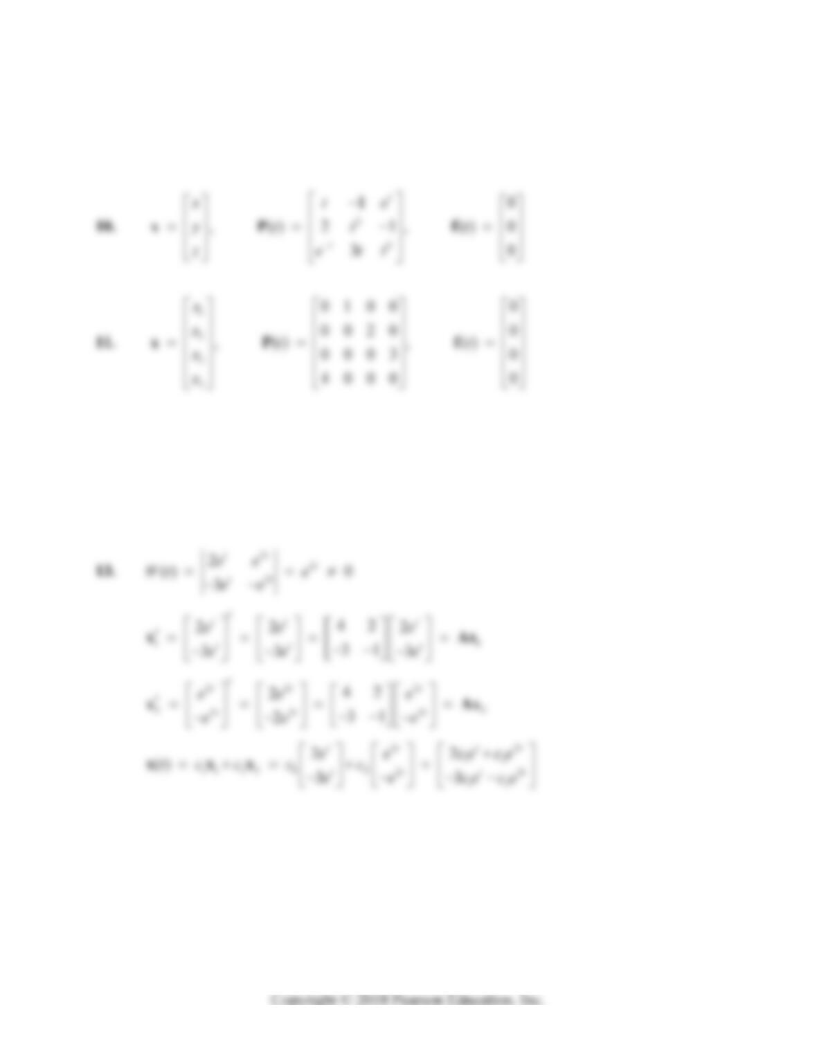
7.
011 0
,()101,()0
110 0
x
yt t
z
xP f
390 Chapter 7: Linear Systems of Differential Equations
9. 2
3
341
,()103,()
06 7
x
t
yt tt
zt
xP f
12.
1
2
2
3
3
4
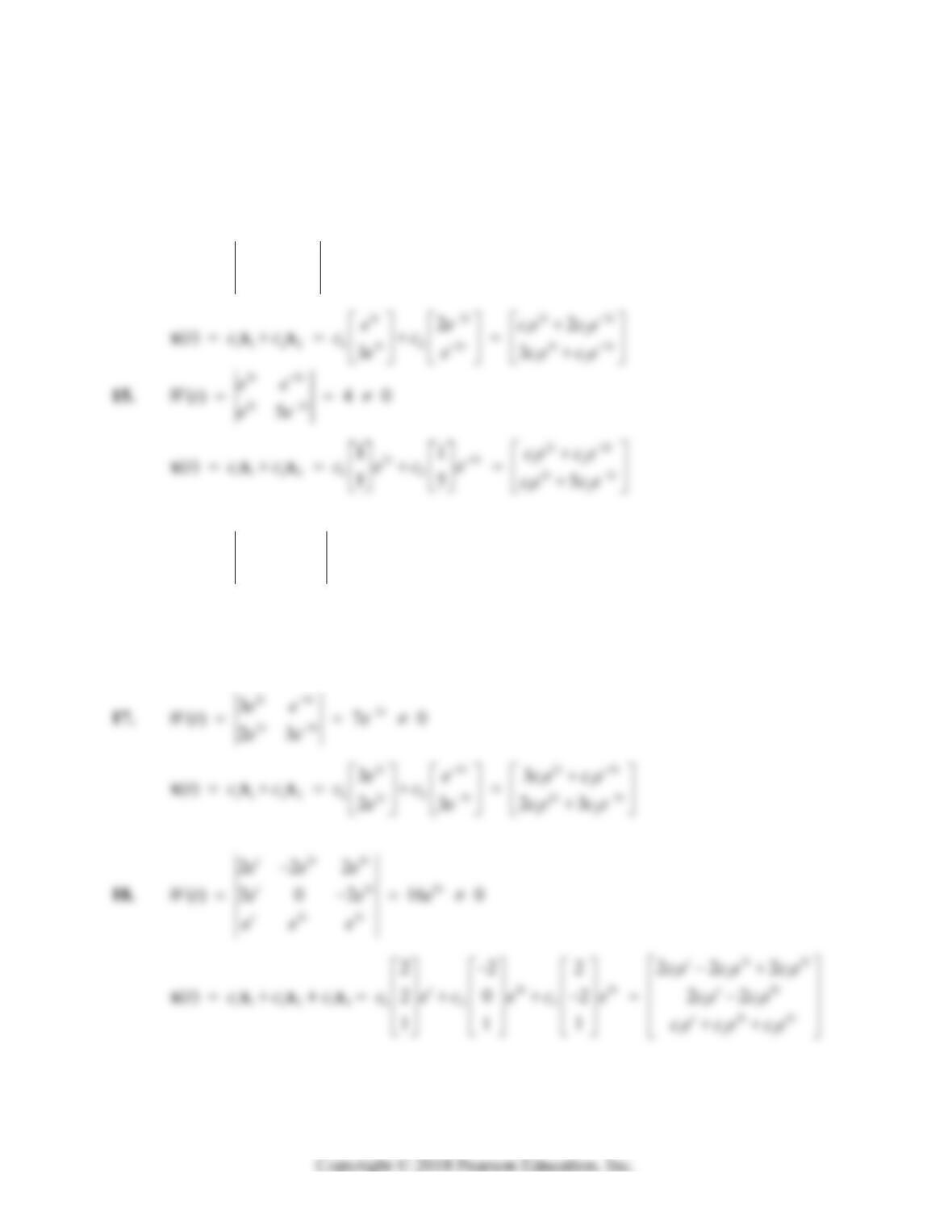
0110 0
0011
,() ,()
1001
1100
x
xt
tt
xt
xt
xP f
Section 7.2: Matrices and Linear Systems 391
In most of Problems 14-22, we omit the verifications of the given solutions. In each case, this is
simply a matter of calculating both the derivative i
x of the given solution vector and the product
i
Ax (where A is the coefficient matrix in the given differential equation) to verify that
ii
xAx (just as in the verification of the solutions 12
andxx in Problem 13 above).
14.
32
3
32
2
() 5 0
3
tt
t
tt
ee
Wt e
ee
16.
32
5
32
() 0
2
tt
t
tt
ee
Wt e
ee
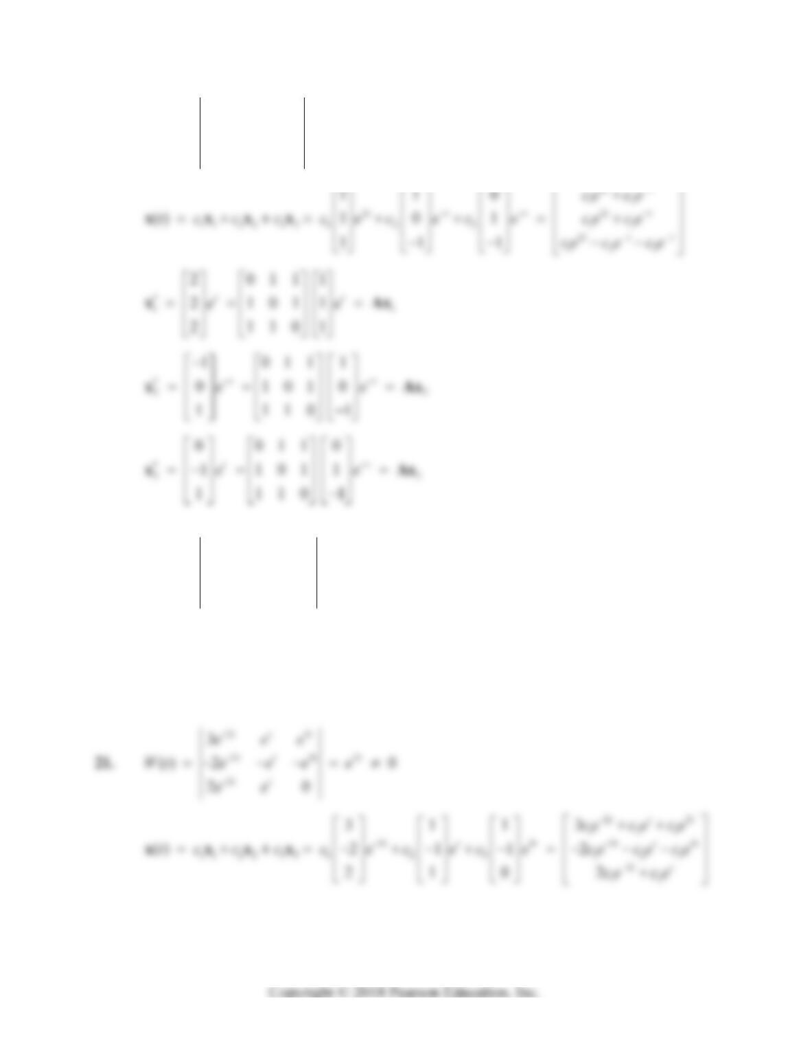
32
32
12
11 2 2 1 2 32
12
11
() 12 2
tt
tt
tt
ce ce
tcc c ec e ce c e
xxx
392 Chapter 7: Linear Systems of Differential Equations
19.
2
2
2
0
() 0 3 0
tt
tt
ttt
ee
Wt e e
eee
20.
34
34 7
34
12
() 6 3 2 84 0
13 2
tt
tt t
tt
ee
Wt e e e
ee
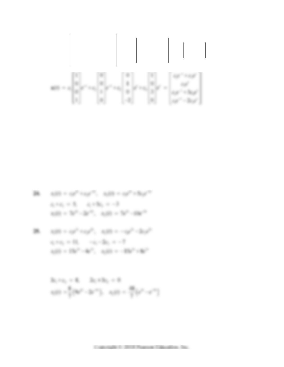
34
12 3
34 34
11 2 2 3 3 1 2 3 1 2 3
34
12 3
12 1 2
() 6 3 2 6 3 2
13 2 1 13 2
tt
tt tt
tt
ccece
tcc c c c ec e ccece
ccece
xxxx
Section 7.2: Matrices and Linear Systems 393
22. 1
00 0
00 0 0
() 0 0 1 0
003 2
20
02 0
tt
tt
tt
tt
tt tt
tt
tt
ee
ee
ee
Wt e e
ee ee
ee
ee
In Problems 23–26 (and similarly in Problems 27–32) we give first the scalar components
12
() and ()
x
txt of a general solution, then the equations in the coefficients 12
andcc that are
obtained when the given initial conditions are imposed, and finally the resulting particular
solution of the given system.
23. 32 32
112 2 12
() 2 , () 3
tt tt
x
tcece xt cece
12 12
32 32
12
20,3 5
() 2 2 , () 6
tt tt
cc cc
x
teextee
x
x
x
x
26. 25 2 5
1122 12
() 3 , () 2 3
tt t t
x
tcecextcece
x
394 Chapter 7: Linear Systems of Differential Equations
27. 35 5 35
11232133123
()22 2,()22,()
ttt tt ttt
x
tcececextcecextcecece
123 13 123
35 5 35
123
2220,220, 4
() 2 4 2 , () 2 2 , () 2
ttt tt ttt
cc c cc ccc
x
teeexteexteee
x
x
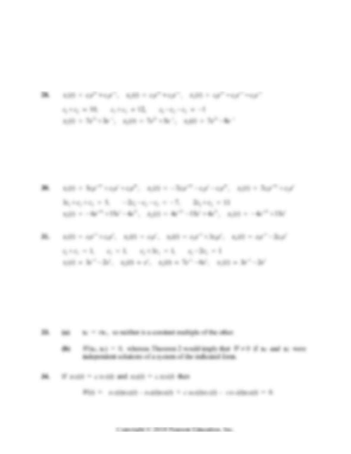
29. 23 23 2
11232 1233 12
()3,()2,()2
tt t tt t tt
x
t cececext cececext cece
123 123 12
23 23 2
12 3
31,2 2,23
() 9 3 5 , () 6 3 5 , () 6 3
tt t tt t tt
ccc ccc cc
x
teeext eeextee
x
x
x
x
32. 1142 33 24413
() , () , () 3 , () 2
tt t t t t t
x
tcecextcextcecextce ce
14 3 2 4 1 3
123 4
1, 3, 3 4, 2 7
( ) 13 12 , ( ) 3 , ( ) 40 36 , ( ) 13 6
tt t t t tt
cc c c c c c
x
teextext eextee