CHAPTER 5
LINEAR EQUATIONS OF HIGHER ORDER
SECTION 5.1
INTRODUCTION: SECOND-ORDER LINEAR EQUATIONS
In this section the central ideas of the theory of linear differential equations are introduced and
illustrated concretely in the context of second-order equations. These key concepts include su-
perposition of solutions (Theorem 1), existence and uniqueness of solutions (Theorem 2), linear
1. Imposition of the initial conditions
00y,
05y on the general solution
x
x
5
2. Imposition of the initial conditions
01y ,
015y on the general solution
3. Imposition of the initial conditions
03y,
08y on the general solution
4. Imposition of the initial conditions
010y,
010y on the general solution
276 Chapter 5: Higher-Order Linear Differential Equations
5. Imposition of the initial conditions
01y,
00y on the general solution
x
6. Imposition of the initial conditions
07y,
01y on the general solution
x
7. Imposition of the initial conditions
02y ,
08y on the general solution
x
8. Imposition of the initial conditions
04y,
02y on the general solution
9. Imposition of the initial conditions
02y,
01y on the general solution
x
10. Imposition of the initial conditions
03y,
013y on the general soution
x
11. Imposition of the initial conditions (0) 0y,
05y on the general solution
xx
12. Imposition of the initial conditions
02y,
00y on the general solution
Section 5.1: Introduction: Second-Order Linear Equations 277
13. Imposition of the initial conditions
13y,
11y on the general solution
14. Imposition of the initial conditions
210y,
215y on the general solution
c
3
c
x
15. Imposition of the initial conditions
17y,
12y on the general solution
16. Imposition of the initial conditions
12y,
13y on the general solution
17. If c
y
x
, then
2
2
22 2
10
cc
cc
yy xx x
unless either 0c or 1c.
18. If 3
y
cx, then 3244
66 6
y
ycxcx cx x
unless 21c.
21. Linearly independent, because 32
x
xx if 0x, whereas 32
x
xx if 0x.
22. Linearly independent, because
11
x
cx would require that 1c with 0x, but
278 Chapter 5: Higher-Order Linear Differential Equations
26. To see that
f
x and
gx are linearly independent, assume that
f
xcgx, and
then substitute both 0x and 2
x
.
29. There is no contradiction, because if the given differential equation is divided by 2
x
to
get the form in Equation (8) in the text, then the resulting functions
4
px
x
and
2
6
qx
x
are not continuous at 0x.
30. (a) 3
1
y
x and 3
2
yx are linearly independent because 33
x
cx would require that
1c with 1x, but 1c with 1x .
y
y
y
33
xx
x
x
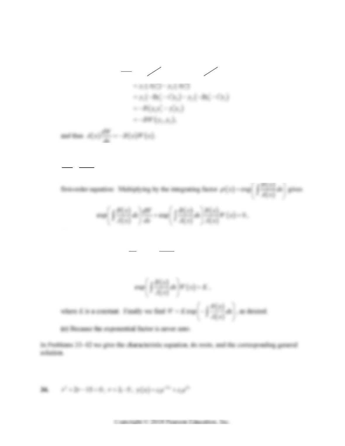
31.
12
,2Wyy x vanishes at 0x, whereas if 1
y
and 2
y
were (linearly independent)
Section 5.1: Introduction: Second-Order Linear Equations 279
32. (a) Because 12 12
Wyy yy
, we have
12
dW
AAyy
dx
12 12 12
yy yy yy
(b) The differential equation for
Wx found in a can be rewritten as
0
Bx
dW Wx
dx A x
, since
Ax is never zero. We can solve this equation as a linear
or
exp 0
Bx
ddx W x
dx A x
,
or
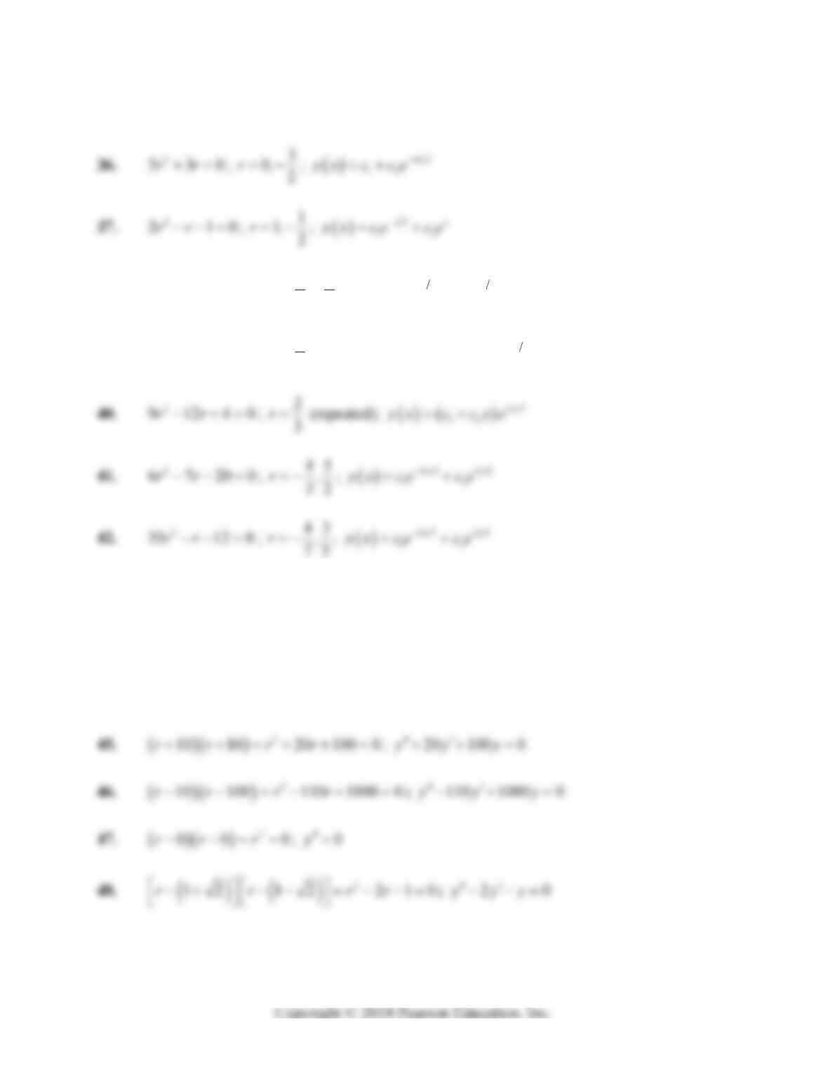
33. 2320rr; 1,2r;
2
12
x
x
y
xcece
280 Chapter 5: Higher-Order Linear Differential Equations
35. 250rr; 0, 5r;
5
12
x
y
xcce
x
x
y
38. 2
4830rr
; 13
,
22
r ;
232
12
x
x
yx ce ce
39. 2
4410rr; 1
2
r (repeated);
2
12
x
y
xccxe
x
y
x
y
x
y
In Problems 43–48 we first write and simplify the equation with the indicated characteristic
roots, and then write the corresponding differential equation.
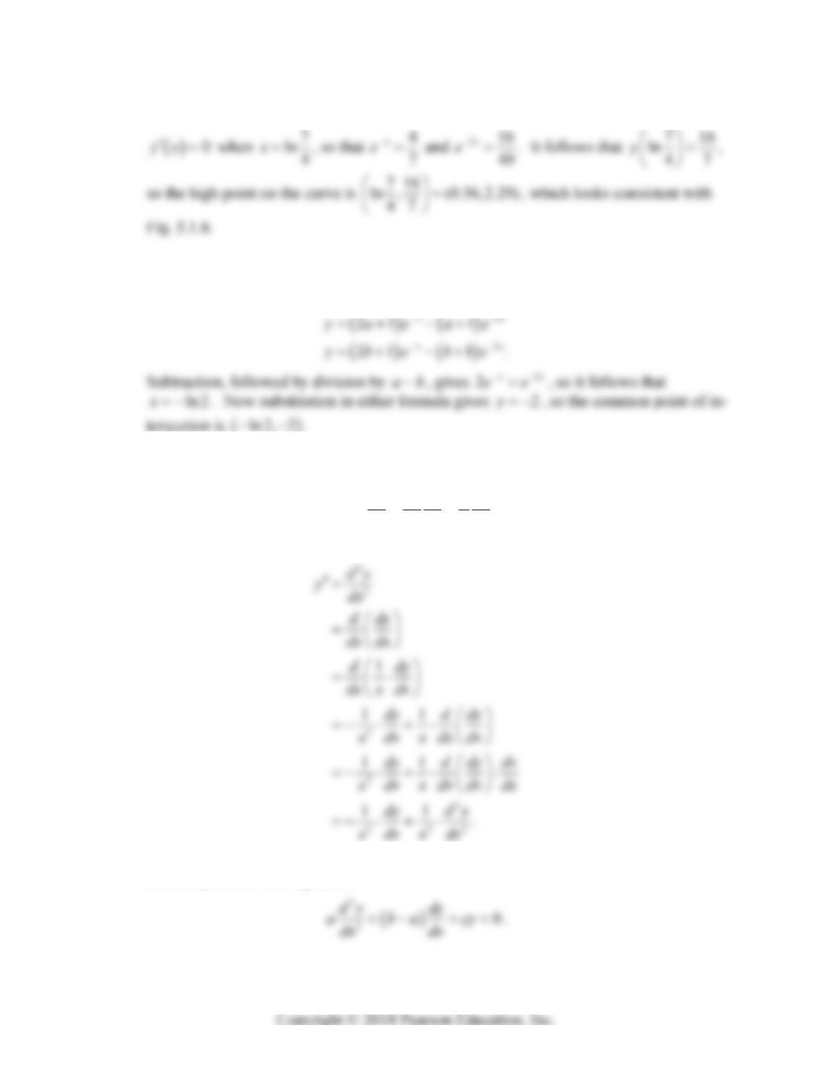
43.
2
010 100rr rr; 10 0yy
44.
2
10 10 100 0rr r
; 100 0
y
y
Section 5.1: Introduction: Second-Order Linear Equations 281
49. The solution curve with
01y,
06y is
2
87
x
x
y
xe e
. We find that
50. The two solution curves satisfying
0
y
a and
0
y
b, as well as
01y, are giv-
en by
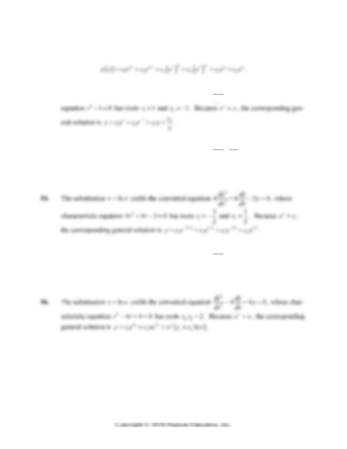
51. (a) The substitution lnvx gives
1dy dy dv dy
ydx dv dx x dv
.
Then another differentiation using the chain and product rules gives
Substitution of these expressions for y and y into Eq. (21) in the text then yields im-
mediately the desired Eq. (23):
282 Chapter 5: Higher-Order Linear Differential Equations
(b) If the roots
1
r and
2
r of the characteristic equation of Eq. (23) are real and distinct,
then a general solution of the original Euler equation is
y
52. The substitution lnvx yields the converted equation
2
20
dy y
dv , whose characteristic
53. The substitution lnvx yields the converted equation
2
212 0
dy dy y
dv dv
, whose char-
acteristic equation 212 0rr has roots 14r and 23r. Because v
ex, the cor-
responding general solution is 43 43
1212
vv
y
ce ce cx c x
.
55. The substitution lnvx yields the converted equation
2
20
dy
dv , whose characteristic
equation 20r has repeated roots 12
,0rr. Because lnvx, the corresponding general
solution is 12 12
ln
y
ccvcc x .
SECTION 5.2
GENERAL SOLUTIONS OF LINEAR EQUATIONS
Students should check each of Theorems 1 through 4 in this section to see that, in the case 2n,
it reduces to the corresponding theorem in Section 5.1. Similarly, the computational problems
for this section largely parallel those for the previous section. By the end of Section 5.2 students
Section 5.2: General Solutions of Linear Equations 283
The linear combinations listed in Problems 1–6 were discovered “by inspection”—that is, by trial
and error.
1.
22
58
231580
23
xxxx
for all x.
2.
22
4 5 5 2 3 1 10 15 0xx for all x.
6.
11cosh1sinh0
x
exx , because
1
cosh 2
x
x
x
ee
and
1
sinh 2
x
x
x
ee
.
x
11. 32
x
Wxe is nonzero if 0x.
12.
22 2 2
2cos ln 2sin ln 2Wx x x x
is nonzero for 0x.
284 Chapter 5: Higher-Order Linear Differential Equations
y
y
y
13. Imposition of the initial conditions
01y,
02y,
00y on the general solu-
tion
2
12 3
x
xx
y
xcece ce
yields the three equations
14. Imposition of the initial conditions
00y,
00y,
03y on the general solu-
tion
23
12 3
x
xx
y
xcece ce yields the three equations
x
15. Imposition of the initial conditions
02y,
00y,
00y on the general solu-
tion
2
12 3
x
xx
y
xcecxecxe yields the three equations
x
16. Imposition of the initial conditions
01y,
04y,
00y on the general solu-
tion
22
12 3
x
xx
y
xcece cxe yields the three equations
x
y
17. Imposition of the initial conditions
03y,
01y,
02y on the general solu-
tion
12 3
cos3 sin 3
y
xcc xc x yields the three equations
Section 5.2: General Solutions of Linear Equations 285
18. Imposition of the initial conditions
01y,
00y,
00y on the general solu-
tion
12 3
cos sin
x
y
xecc xc x yields the three equations
y
19. Imposition of the initial conditions
16y,
114y,
122y on the general solu-
tion
23
12 3
y
xcxcxcx yields the three equations
y
20. Imposition of the initial conditions
11y,
15y,
111y on the general solu-
tion
22
12 3
ln
y
xcxcx cx x
yields the three equations
y
y
y
21. Imposition of the initial conditions
02y,
02y on the general solution
12
cos sin 3
y
xc xc xx yields the two equations 12c, 232c with solution
286 Chapter 5: Higher-Order Linear Differential Equations
22. Imposition of the initial conditions
00y,
010y on the general solution
23. Imposition of the initial conditions
03y,
011y on the general solution
24. Imposition of the initial conditions
04y,
08y on the general solution
xx
25.
12 1 2
Ly L y y Ly Ly f g
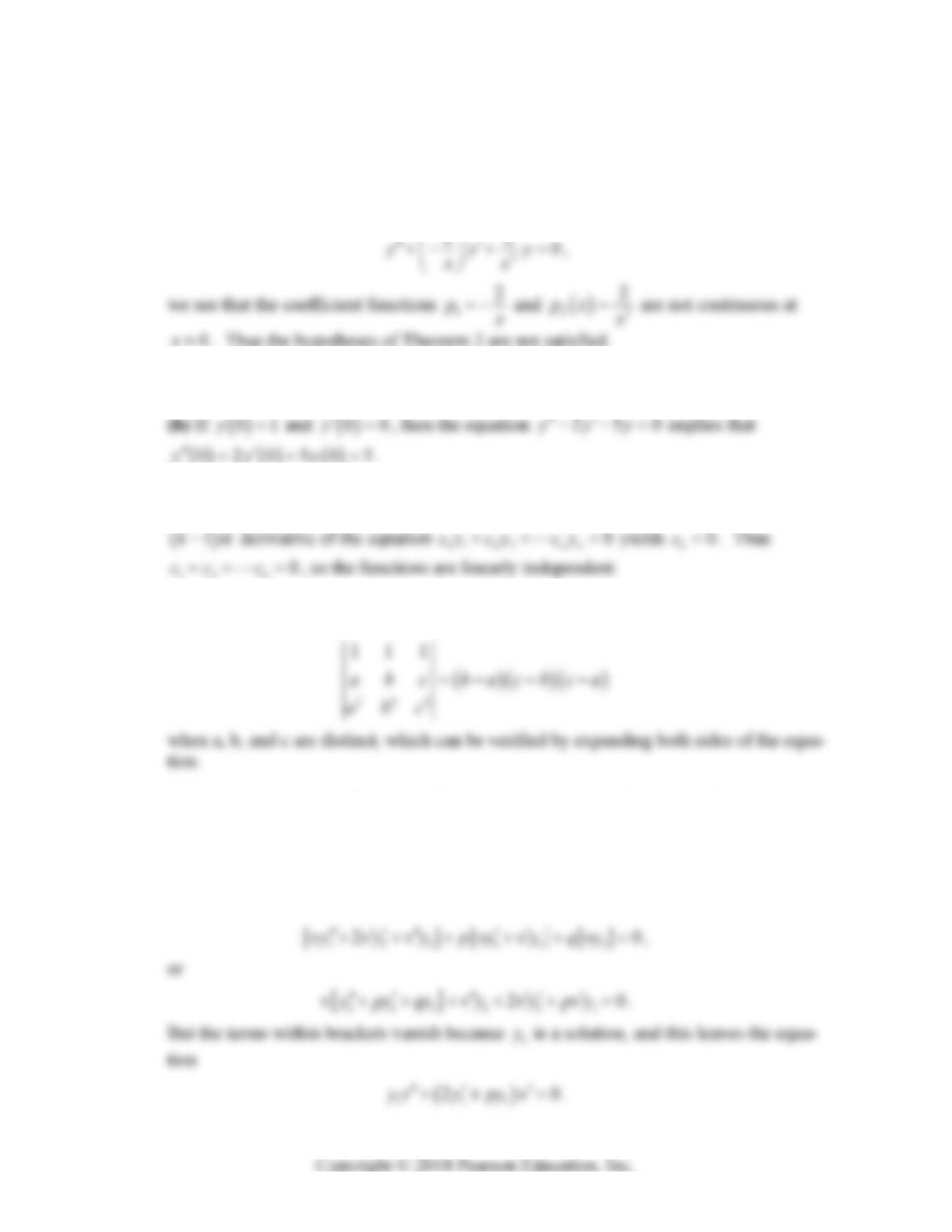
27. The equations
28. If we differentiate the equation 2
01 2 0
n
n
ccxcx cx repeatedly, n times in suc–
cession, the result is the system
2
01 2
0
n
n
ccxcx cx
Section 5.2: General Solutions of Linear Equations 287
29. If
01 0
rx rx n rx
n
ce cxe cx e , then division by rx
e yields 01 0
n
n
ccx cx , so
the result of Problem 28 applies.
30. When the equation 2
220xy xy y
is rewritten in standard form
31. (a) Substitution of
x
a in the differential equation gives
y
apyaqa
.
32. Let the functions 12
,,,
n
y
yy be chosen as indicated. Then evaluation at
x
a of the
33. This follows from the fact that
34.
12 1
,,, exp n
ni
i
Wff f V rx
, and neither V nor
1
exp n
i
irx
vanishes.
36. If 1
y
vy, then substitution of the derivatives 11
y
vy v y
, 111
2
y
vy v y v y
in the
differential equation 0ypyqy
gives
y
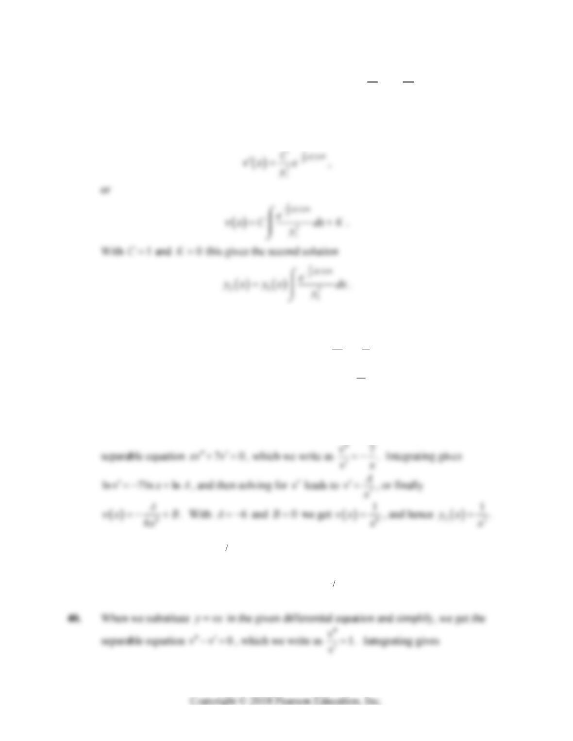
288 Chapter 5: Higher-Order Linear Differential Equations
We can solve this by separating variables and integrating: 1
1
2
vy
p
vy
leads to
1
ln 2ln lnvypxdxC
,
or
y
37. When we substitute 3
y
vx in the given differential equation and simplify, we get the
separable equation 0xv v
, which we write as 1v
vx
. Integrating gives
ln ln lnvxA
, and then solving for v leads to
A
v
x
, or finally
lnvx A x B
.
With 1
A
and 0B we get
lnvx x, and thus
3
2ln
y
xxx.
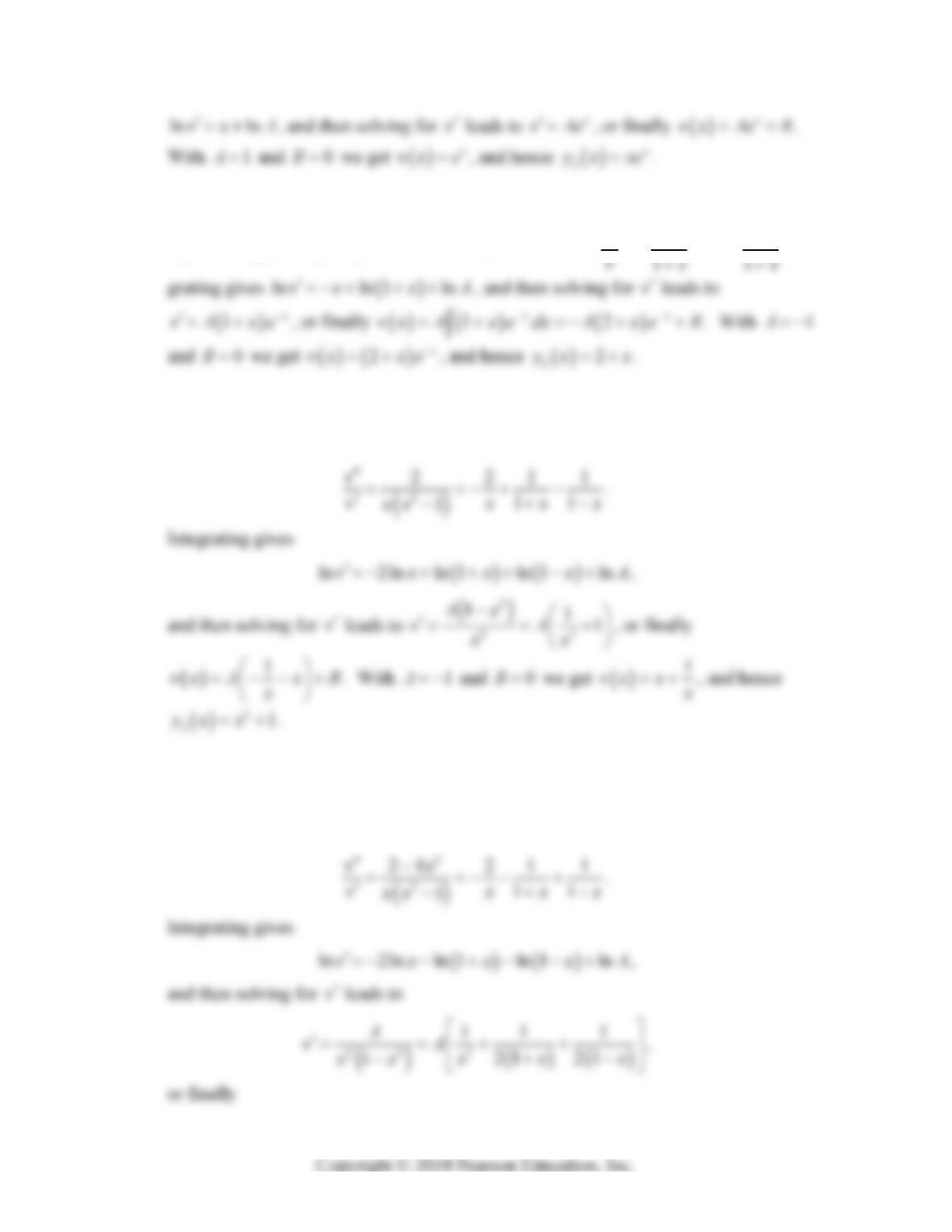
38. When we substitute 3
y
vx in the given differential equation and simplify, we get the
x
x
x
39. When we substitute 2
x
y
ve in the given differential equation and simplify, we eventu-
ally get the simple equation 0v , with general solution
vx Ax B
. With 1A
and 0B we get
vx x, and hence
2
2
x
y
xxe.
Section 5.2: General Solutions of Linear Equations 289
x
x
x
41. When we substitute
x
y
ve in the given differential equation and simplify, we get the
separable equation
10xv xv
, which we write as 1
1
x
x
vx
. Inte-
42. When we substitute
y
vx in the given differential equation and simplify, we get the
separable equation
212
x
xvv
, which we write as
x
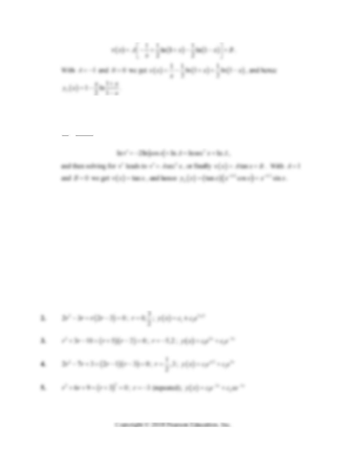
43. When we substitute
y
vx in the given differential equation and simplify, we get the
separable equation
22
124
x
xv xv
, which we write using the method of partial
fractions as
290 Chapter 5: Higher-Order Linear Differential Equations
44. When we substitute 1/2 cos
y
vx x
in the given differential equation and simplify, we
eventually get the separable equation
cos 2 sin
x
vxv
, which we write as
2sin
cos
vx
vx
. Integrating gives
SECTION 5.3
HOMOGENEOUS EQUATIONS WITH CONSTANT COEFFICIENTS
This is a purely computational section devoted to the single most widely applicable type of high-
er order differential equations—linear ones with constant coefficients. In Problems 1–20, we
first write the characteristic equation and list its roots, then give the corresponding general solu-
tion of the given differential equation. Explanatory comments are included only when the solu-
tion of the characteristic equation is not routine.
1.
24220rrr ; 2,2r ;
22
12
x
x
y
xce ce
y
y
y
y
Section 5.3: Homogeneous Equations with Constant Coefficients 291
6. 2550rr
; 55
2
r
;
55 55
22
12
x
x
yx ce ce
x
y
y
y
10.
433
53 530rrrr
; 3
0, 0, 0, 5
r;
235
12 3 4
x
yx c cx cx ce
11.
2
43 22
816 4 0rr rrr ; 0, 0, 4,4r;
44
12 3 4
x
x
y
x c cx ce cxe
12.
3
432
33 10rrrrrr
; 0,1,1,1r;
2
12 3 4
x
xx
y
xccecxecxe
x
y
x
16.
2
42 2
18 81 9 0rr r; 3 , 3rii ;
12 34
cos3 sin 3yx c cx x c cx x
17.
42 2 2
611421340rr r r ; 2
,
23
ii
r ;
292 Chapter 5: Higher-Order Linear Differential Equations
19. Factoring by grouping gives
2
32 2 2
111110rrr rr r r r ;
1, 1, 1r;
12 3
x
xx
y
xcece cxe
.
21. Imposition of the initial conditions
07y,
011y on the general solution
3
12
x
x
y
xcece yields the two equations 12
7cc, 12
311cc with solution
15c, 22c. Hence the desired particular solution is
3
52
x
x
y
xee .
23. Imposition of the initial conditions
03y,
01y on the general solution
3
12
cos4 sin 4
x
y
xec xc x yields the two equations 13c, 12
34 1cc with solu-
tion 13c, 22c . Hence the desired particular solution is
33cos4 2sin4
x
y
xe x x
.
24. Imposition of the initial conditions
01y,
01y ,
03y on the general solu-
x
y
x
Section 5.3: Homogeneous Equations with Constant Coefficients 293
25. Imposition of the initial conditions
01y ,
00y,
01y on the general solu-
tion
23
12 3
x
yx c cx ce
yields the three equations
26. Imposition of the initial conditions
01y,
01y ,
03y on the general solu-
tion
55
12 3
x
x
y
xcce cxe
yields the three equations
27. First we spot the root 1r. Then long division of the polynomial 32
34rr
by 1r
y
28. First we spot the root 2r. Then long division of the polynomial 32
252rr r by
y
29. First we spot the root 3r . Then long division of the polynomial 327r by 3r
yields the quadratic factor 239rr
, with roots 333
22
ri . Hence the general solu-
30. First we spot the root 1r . Then long division of the polynomial 432
36rrr r
by 1r yields the cubic factor 32
236rrr
. Next we spot the root 2r, and anoth-
294 Chapter 5: Higher-Order Linear Differential Equations
31. The characteristic equation 32
3480rrr has the evident root 1r, and long divi-
y
32. The characteristic equation 43 2
3520rr r r has the root 2r, as is readily
found by trial and error, and long division then yields the factorization
33. Knowing that 3
x
y
e is one solution, we divide the characteristic polynomial
y
34. Knowing that 23
x
y
e is one solution, we divide the characteristic polynomial
y
35. The fact that cos2yx is one solution tells us that 24r is a factor of the characteristic
polynomial 43 2
6 5 25 20 4rr r r . Then long division yields the quadratic factor
y
36. The fact that sin
x
y
ex
is one solution tells us that
22
11 22rrr is a factor
y
37. The characteristic equation is
43 3 10rrrr , so the general solution is
2
x
y
xABxCxDe . Imposition of the given initial conditions yields the equa-
tions
x