Section 2.1: Population Models 115
15
20
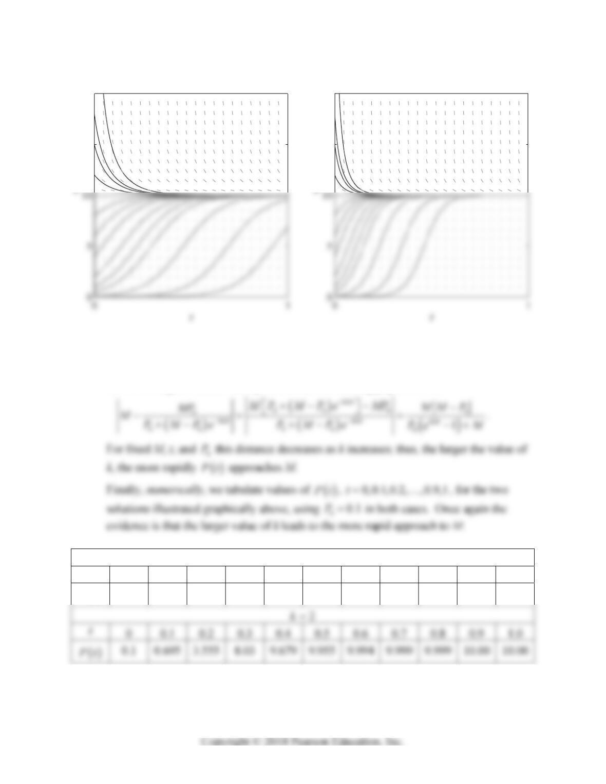
Problem 35 (k = 1)
15
20
Problem 35 (k = 2)
These diagrams suggest that the larger the value of k, the more rapidly the population
Pt approaches the limiting population M.
To look at things analytically, we examine the distance between the solution (7) in the
text of the logistic initial value problem and the limiting population M:
1k
t 0 0.1 0.2 0.3 0.4 0.5 0.6 0.7 0.8 0.9 1.0
Pt 0.1 0.267 0.695 1.687 3.555 5.999 8.030 9.172 9.679 9.879 9.955
116 Chapter 2: Mathematical Models and Numerical Methods
36. With 50kM
xe
, 05.308P, 123.192P, and 276.212P, Equation (7) in the text takes
the forms
00
from which we get
0
00
1
20
00
2
PM
PMPx P
PM
PMPx P
,
Expanding gives
222222
02 012 01 2 1 1 0 2 01 2
2PPM PPPM PPP PM P P P M PPP
,
in which we cancel the final term on each side and solve for
(ii)
1020112
2
02 1
2PPPPPPP
MPP P
.
Section 2.2: Equilibrium Solutions and Stability 117
In Problems 37 and 38 we give just the values of k and M calculated using Equations (ii) and (iii)
in Problem 36 above, the resulting logistic solution, and the predicted year 2000 population.
39. Separating variables gives
1cos2dP k b t dt
P
, or
ln sin 2
2
b
Pkt tC
. The initial
condition
0
0PP implies that 0
lnCP,
SECTION 2.2
EQUILIBRIUM SOLUTIONS AND STABILITY
In Problems 1-12 we identify the stable and unstable critical points as well as the funnels and
spouts along the equilibrium solutions. In each problem the indicated solution satisfying
0
0
x
x is derived by separation of variables, and we show typical solution curves
corresponding to different values of 0
x
.
110
115
120
P
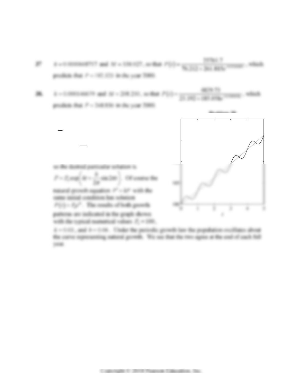
Problem 39
118 Chapter 2: Mathematical Models and Numerical Methods
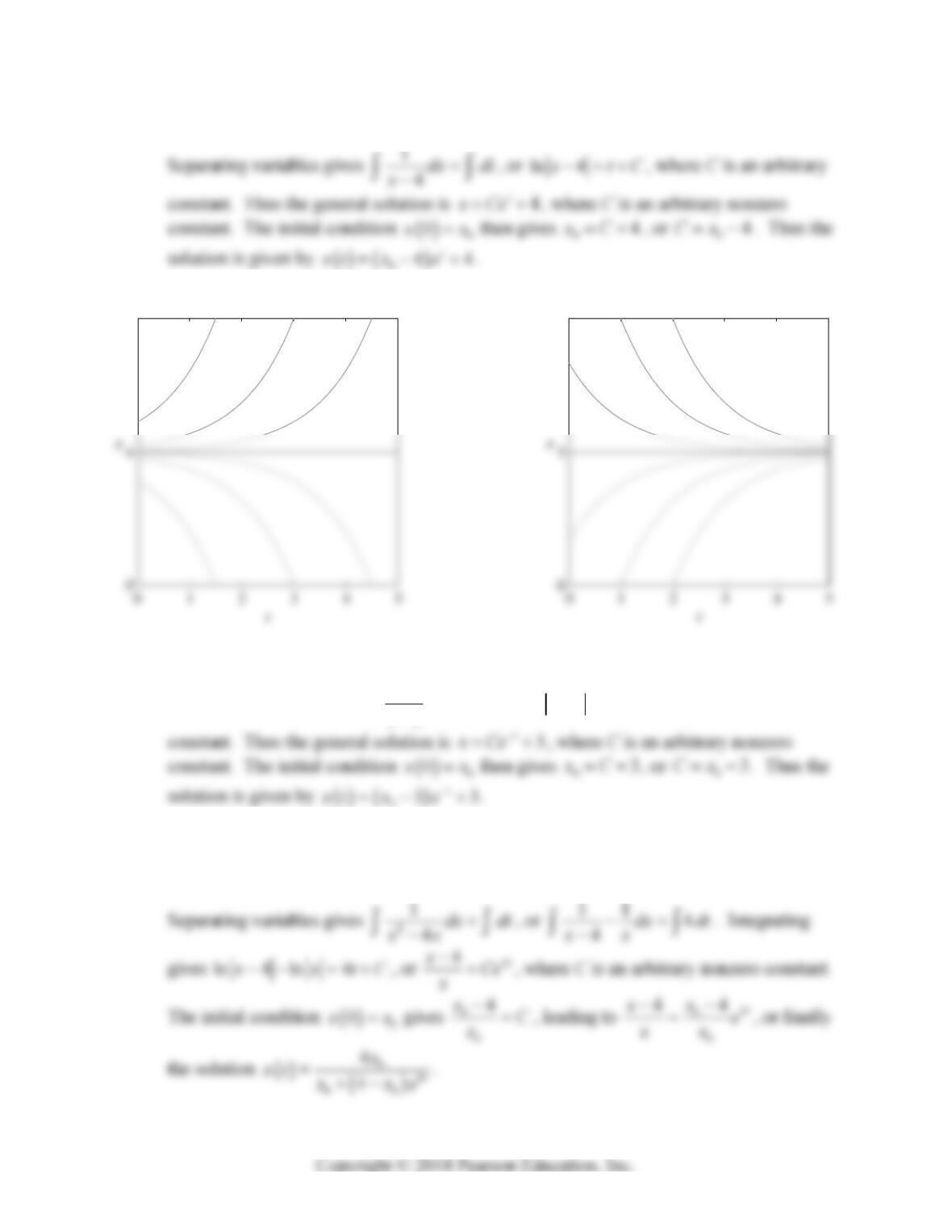
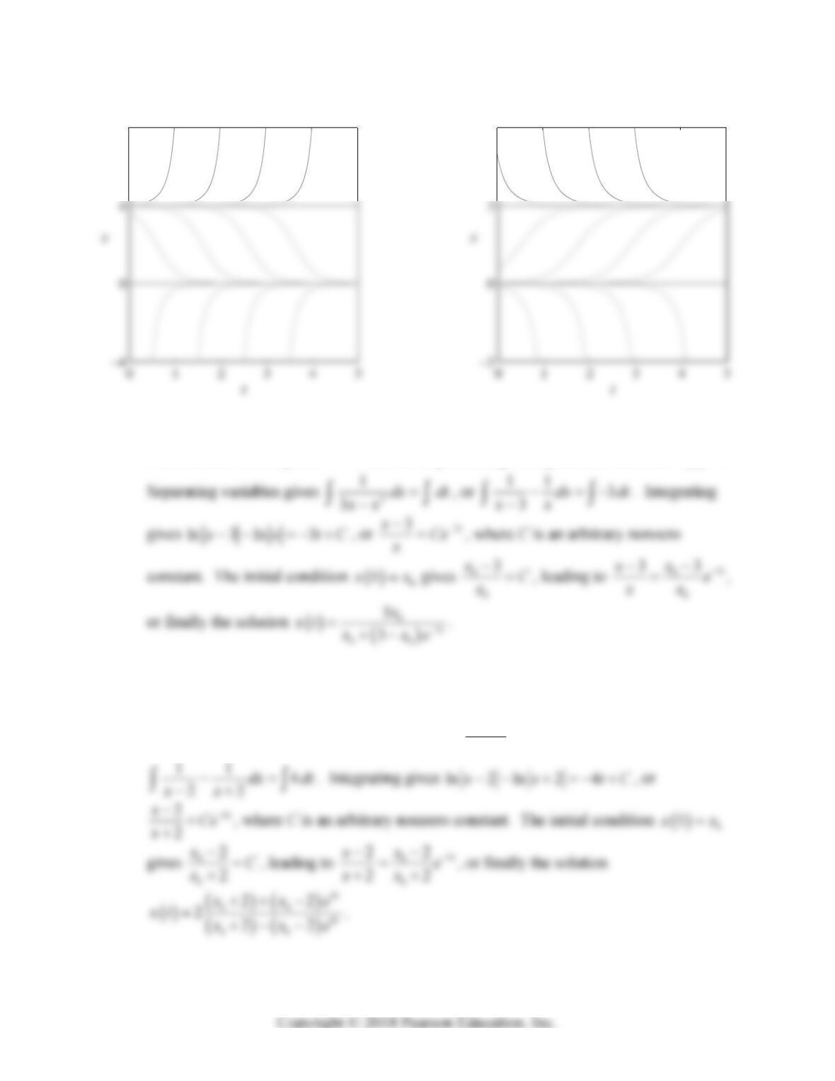
1. The unstable critical point 4x leads to a spout along the equilibrium solution
4xt .
8
Problem 1
6
Problem 2
2. The stable critical point 3x leads to a funnel along the equilibrium solution
4xt .
Separating variables gives 1
3dx dt
x
, or ln 3
x
tC, where C is an arbitrary
033
3. The stable critical point 0x leads to a funnel along the equilibrium solution
0xt .
The unstable critical point 4x leads to a spout along the equilibrium solution
4xt .
Section 2.2: Equilibrium Solutions and Stability 119
8
Problem 3
6
Problem 4
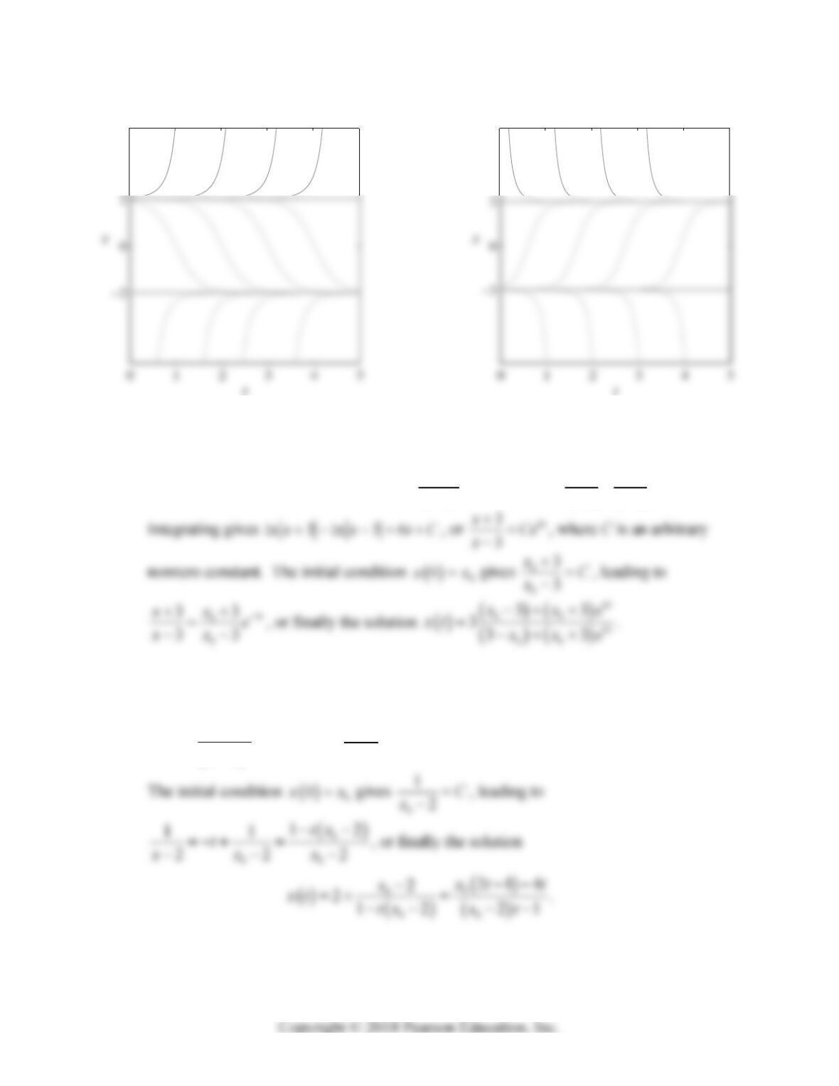
4. The stable critical point 3x leads to a funnel along the equilibrium solution
3xt .
The unstable critical point 0x leads to a spout along the equilibrium solution
0xt .
5. The stable critical point 2x leads to a funnel along the equilibrium solution
2xt . The unstable critical point 2x leads to a spout along the equilibrium
solution
2xt . Separating variables gives 2
1
4dx dt
x
, or
120 Chapter 2: Mathematical Models and Numerical Methods
Problem 5
Problem 6
6. The stable critical point 3x leads to a funnel along the equilibrium solution
3xt .
The unstable critical point 3x leads to a spout along the equilibrium solution
3xt . Separating variables gives 2
1
9dx dt
x
, or 11 6
33
dx dt
xx
.
7. The lone critical point 2x is semi-stable; solutions with 02x approach as t
increases, whereas those with 02x approach 2 as t increases. Separating variables
gives
2
1
2dx dt
x
, or 1
2tC
x
, where C is an arbitrary nonzero constant.
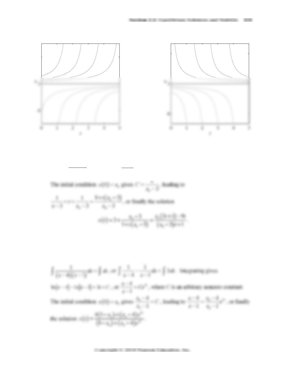
4
Problem 7
6
Problem 8
8. The lone critical point 3x is semi-stable; solutions with 03x approach as t
increases, whereas those with 03x approach 3 as t increases. Separating variables
gives
2
1
3dx dt
x
, or 1
3tC
x
, where C is an arbitrary nonzero constant.
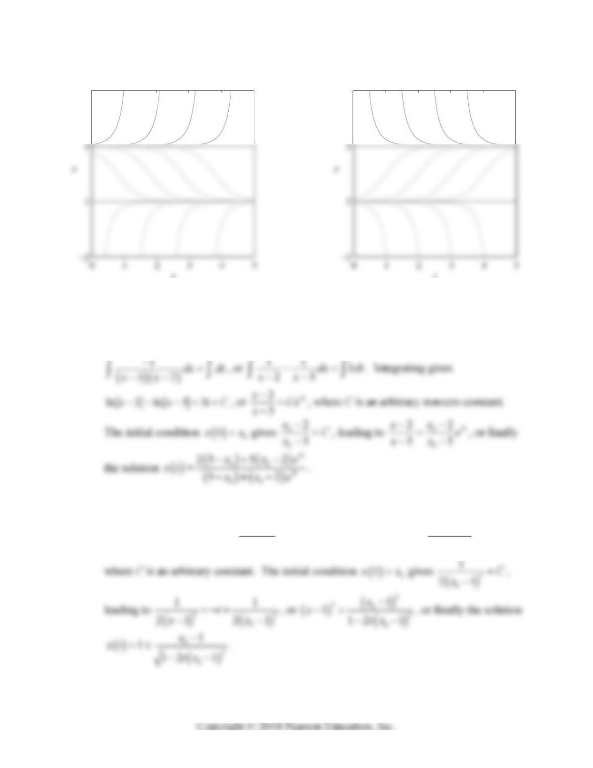
9. Factoring gives
254 4 1xx x x
. The stable critical point 1x leads to a
funnel along the equilibrium solution
1xt . The unstable critical point 4x leads to
a spout along the equilibrium solution
4xt . Separating variables gives
122 Chapter 2: Mathematical Models and Numerical Methods
7
t
Problem 9
8
t
Problem 10
10. Factoring gives
2
710 52xx x x . The stable critical point 5
x
leads to a
funnel along the equilibrium solution
5xt . The unstable critical point 2x leads to
a spout along the equilibrium solution
4xt . Separating variables gives
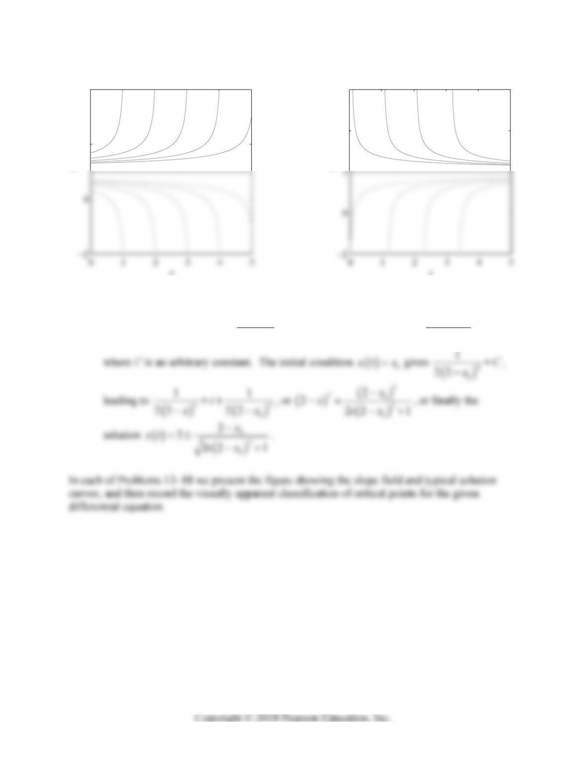
11. The unstable critical point 1x leads to a spout along the equilibrium solution
4xt .
Separating variables gives
3
1
1dx dt
x
, and integrating gives
2
1
21 tC
x
,
Section 2.2: Equilibrium Solutions and Stability 123
2
4
t
x
Problem 11
4
6
t
x
Problem 12
12. The stable critical point 2x leads to a funnel along the equilibrium solution
2xt .
Separating variables gives
3
1
2dx dt
x
, and integrating gives
2
1
22 tC
x
,
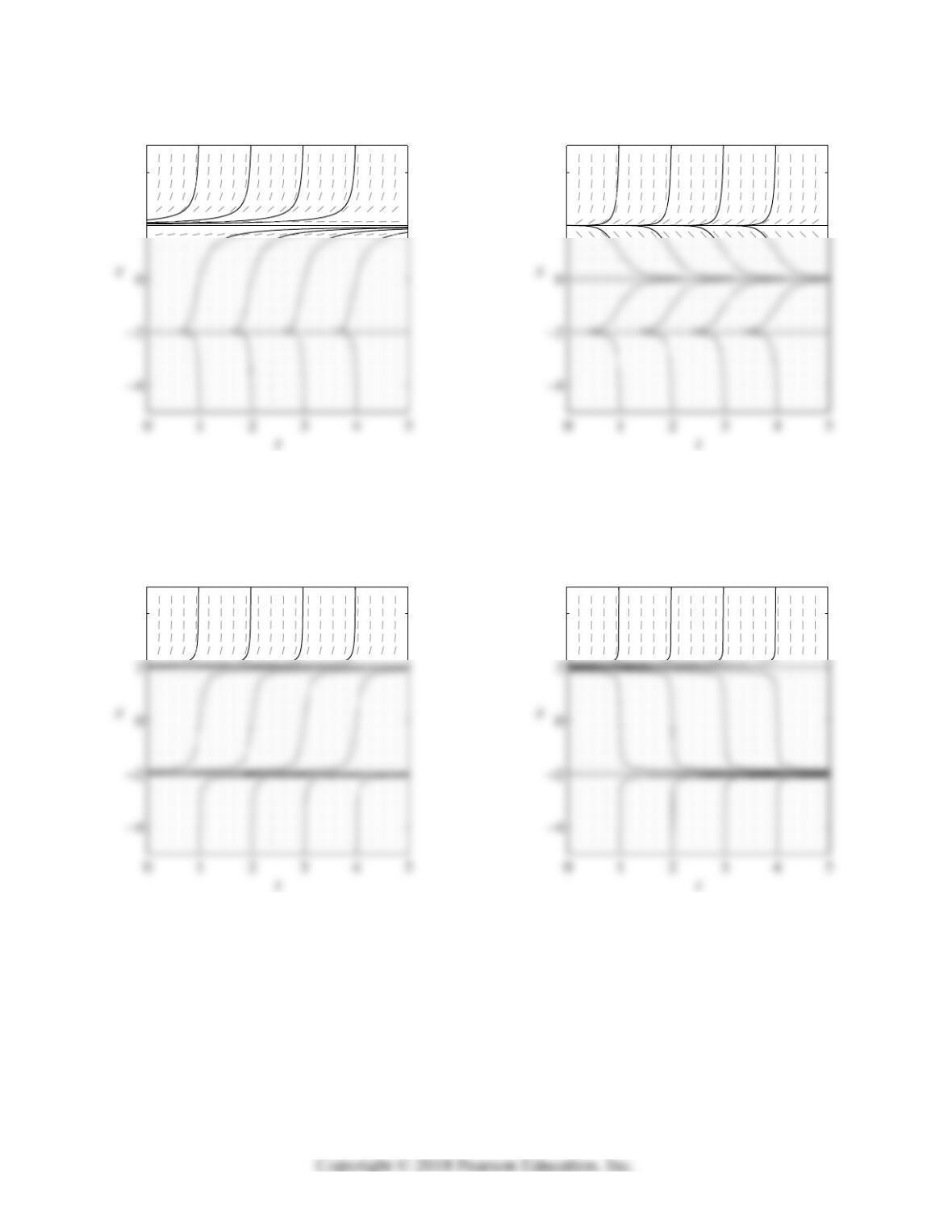
13. The critical points 2x and 2x are both unstable.
124 Chapter 2: Mathematical Models and Numerical Methods
2
4
Problem 13
2
4
Problem 14
14. The critical points 2x are both unstable, whereas the critical point 0x is stable.
15. The critical points 2x and 2x are both unstable.
4
Problem 15
4
Problem 16
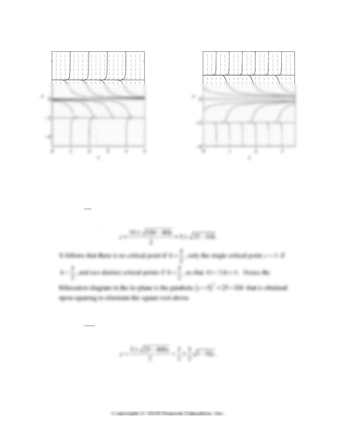
16. The critical point 2x is unstable, while the critical point 2x is stable.
17. The critical points 2x and 0x are unstable, while the critical point 2x is stable.
Section 2.2: Equilibrium Solutions and Stability 125
2
4
Problem 17
2
4
Problem 18
18. The critical points 2x and 2x are unstable, whereas the critical point 0x is
stable.
19. The critical points of the given differential equation are the roots of the quadratic
equation
110 0
10 xxh
, that is,
2
10 10 0xxh
. Thus a critical point c is given
in terms of h by
20. The critical points of the given differential equation are the roots of the quadratic
equation 1(5) 0
100 xx s
, that is, 25 100 0xx s
. Thus a critical point c is given
in terms of s by
126 Chapter 2: Mathematical Models and Numerical Methods
21. (a) If 2
ka , where 0a, then
323 22
0
kx x a x x x a x
only if 0x, so
the only critical point is 0c. If 0a, then we can solve the differential equation by
writing
(b) If 2
ka, where 0a, then
323 0xaxa
kx x a x x x
if either
0x or
x
ak . Thus we have the three critical points 0c and ck ; this
observation, together with part (a), yields the pitchfork bifurcation diagram shown in Fig.
2.2.13 of the textbook. If
00x, then we can solve the differential equation by
writing
x
x
x
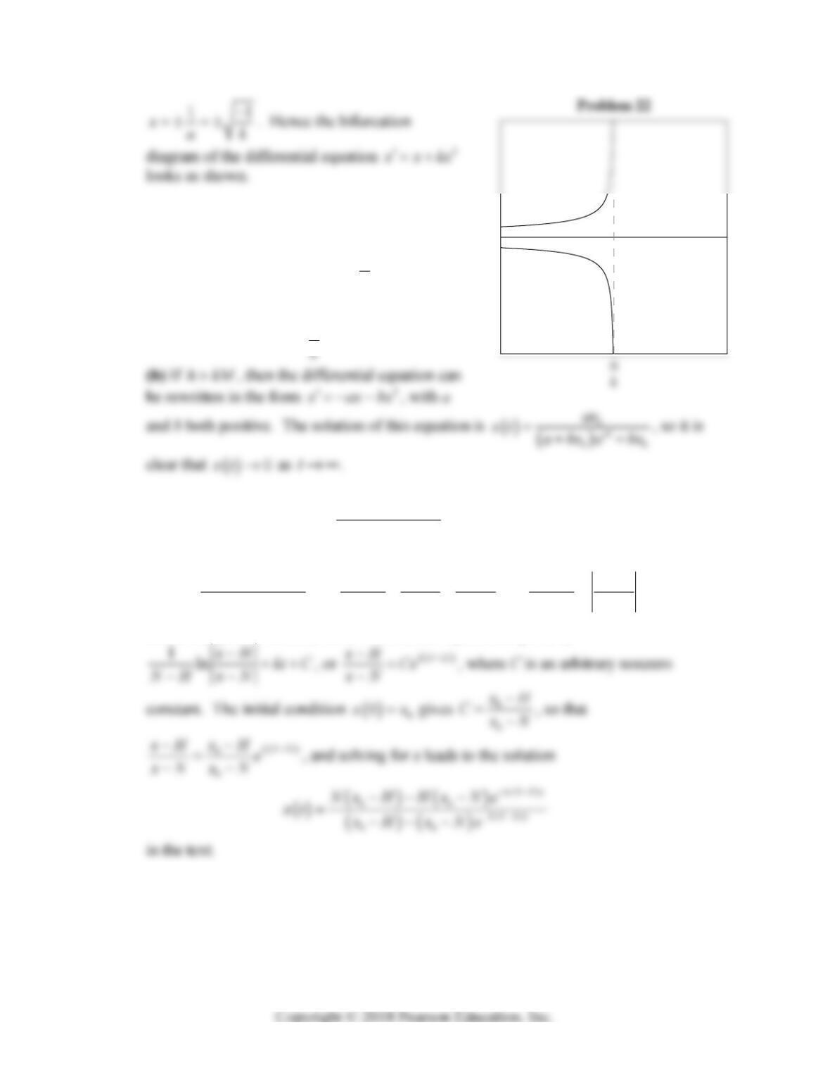
22. If 0k, then the only critical point 0c of the equation
x
x
is unstable, because the
solutions
0
t
x
txe diverge to infinity if 00x. If 20,ka then
Section 2.2: Equilibrium Solutions and Stability 127
23. (a) If hkM, then writing the differential
equation as
h
x
kx M x hx kx M x
k
,
still a logistic equation but with the reduced
limiting population h
Mk
.
24. Separating variables gives
1dx k dt
NxxH
. By the method of partial
fractions,
11111
ln
x
H
dx dx
NxxH NH Nx xH NH xN
,
and so the general solution of the differential equation is given by
x
25. In the first alternative form that is given, all of the coefficients within parentheses are
positive if 0
Hx N. Hence it is clear that
x
tN as t, which confirms (17).
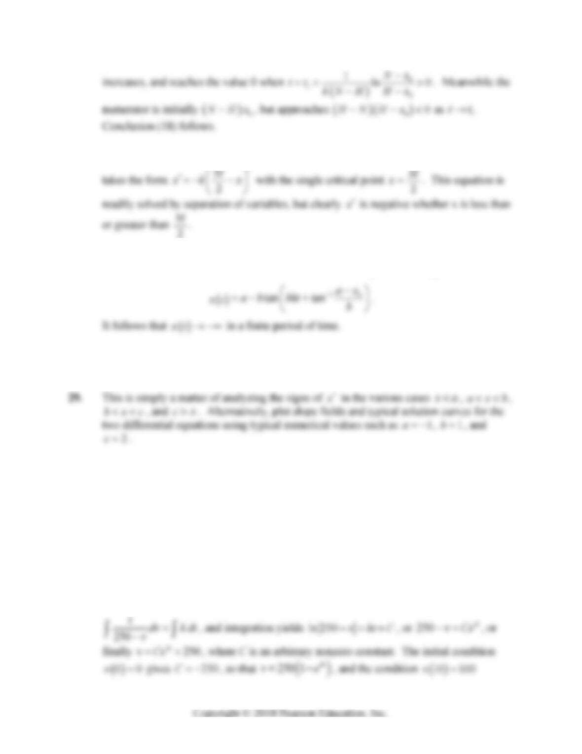
In the second alternative form, all of the coefficients within parentheses are positive if
0
x
H. Hence the denominator is initially equal to 0NH
, but decreases as t
0
c
128 Chapter 2: Mathematical Models and Numerical Methods
26. If 2
4hkM
, then Equations (13) and (14) in the text show that the differential equation
2
27. Separation of variables in the differential equation
22
x
kxa b
yields
28. Aside from a change in sign, this calculation is the same as that indicated in Equations
(13) and (14) in the text.
SECTION 2.3
ACCELERATION-VELOCITY MODELS
This section consists of three essentially independent subsections that can be studied separately:
resistance proportional to velocity, resistance proportional to velocity-squared, and inverse-
square gravitational acceleration.
1. The velocity v of the car (in km/hr) is related to the time t (in seconds) by the initial value
problem
250vk v
,
00v,
10 100v. Separating variables gives
2. (a) The solution of the initial value equation dv kv
dt ,
0
0vv is
0
kt
vt ve
. Then
3. The velocity v of the boat (in ft/s) is related to the time t (in seconds) by the initial value
problem vkv
,
040v,
10 20v. By Problem 2a,
40 kt
vt
, and the
4. Separating variables gives 2
1dv k dt
v
, or 1kt C
v
. The initial condition
0
0vv gives
0
1
Cv
, so that
0
11
kt
vv
, or 0
0
1
11
v
vvkt
kt v
. Then
5. We are assuming that the velocity v of the motorboat satisfies the initial value problem
2
vkv
,
040v, with
10 20v as well. We seek
60x. The result of Problem 4
130 Chapter 2: Mathematical Models and Numerical Methods
6. Separating variables gives 32
1dv k dt
, or 12
2vktC
. The initial condition
Then
0
0
2
0
0
4
4
2
2
v
v
x
dt C
kvkt
vkt
,
and the initial condition
0
0
x
x yields 0
0
2v
x
C
, or 0
0
2v
Cx k
, so that
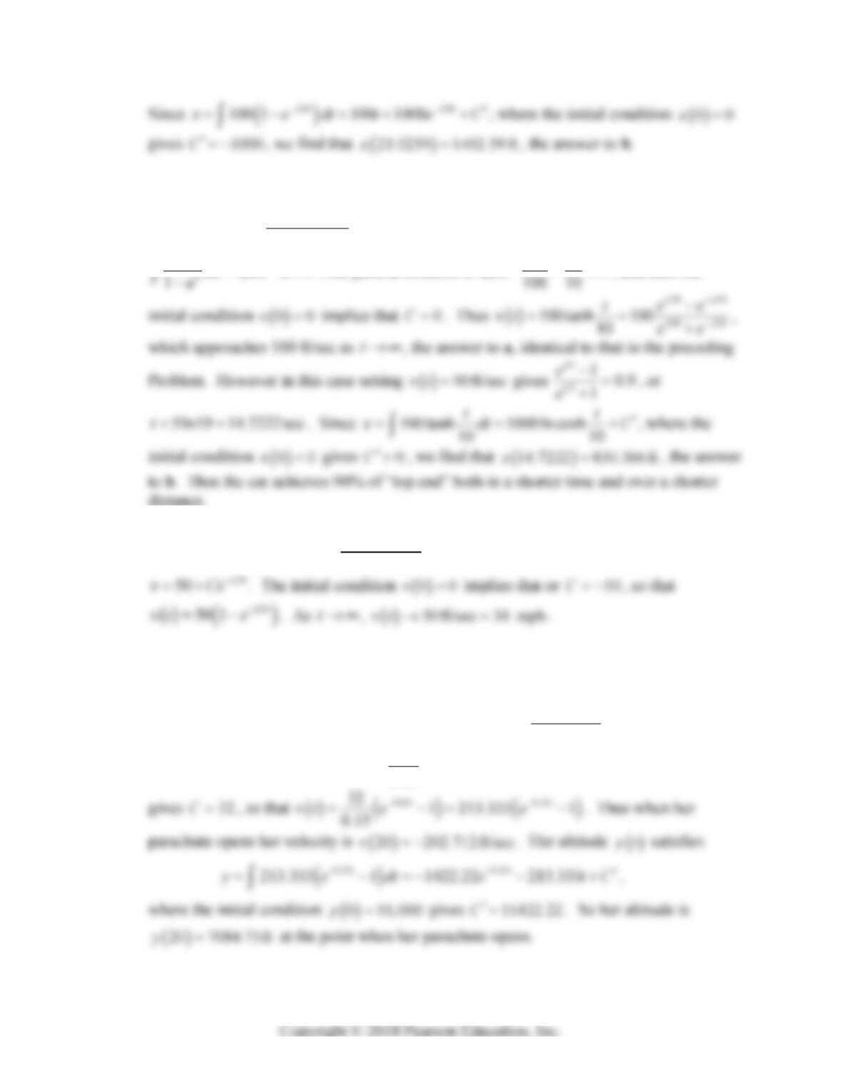
7. The car satisfies the initial value problem 10 0.1vv
,
00v. Separating variables
gives 1
10 0.1 dv dt
v
, or
ln 10 0.1 10
t
vC
. The initial condition
00v
Section 2.3: Acceleration-Velocity Models 131
8. The car now satisfies the initial value problem 2
10 0.001vv
,
00v. Separating
variables gives 2
1
10 0.001 dv dt
v
. By the antiderivative formula
1
1tanh
tanh 100 10
vt
C
, and then the
9. Separating variables gives 1000
5000 100 dv dt
v
, or
10ln 5000 100vtC
, or
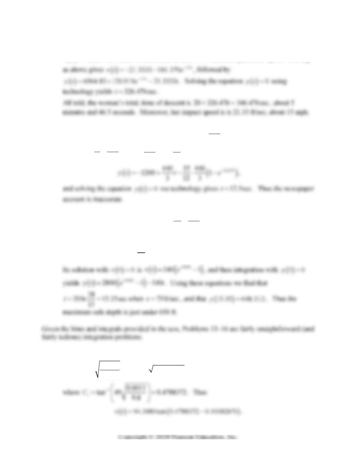
10. We need to solve two initial value problems in succession.
Over the first 20 seconds the woman’s velocity
vt satisfies the initial value problem
32 0.15vv
,
00v. Separating variables gives 1
32 0.15 dv dt
v
, or
ln 32 0.15 0.15vtC
, or
0.15
132
0.15
t
vCe
. The initial condition
00v
132 Chapter 2: Mathematical Models and Numerical Methods
After the parachute opens,
vt satisfies the initial value problem 32 1.5vv
,
0 202.712v , where we reset time so that 0t when the parachute opens. Solving
11. If the paratroopers terminal velocity was 440
100 mph= ft/sec
3, then Equation (7) in the
text yields 440
3
g
, or 312
32
440 55
. Equation (9) then becomes
12. The mass of the drums is given by 640 20slugs
32
W
mg
. With 62.5 8 500lbsB
and lbs
R
Fv , the force equation becomes
20 640 500 140
dv vv
dt .
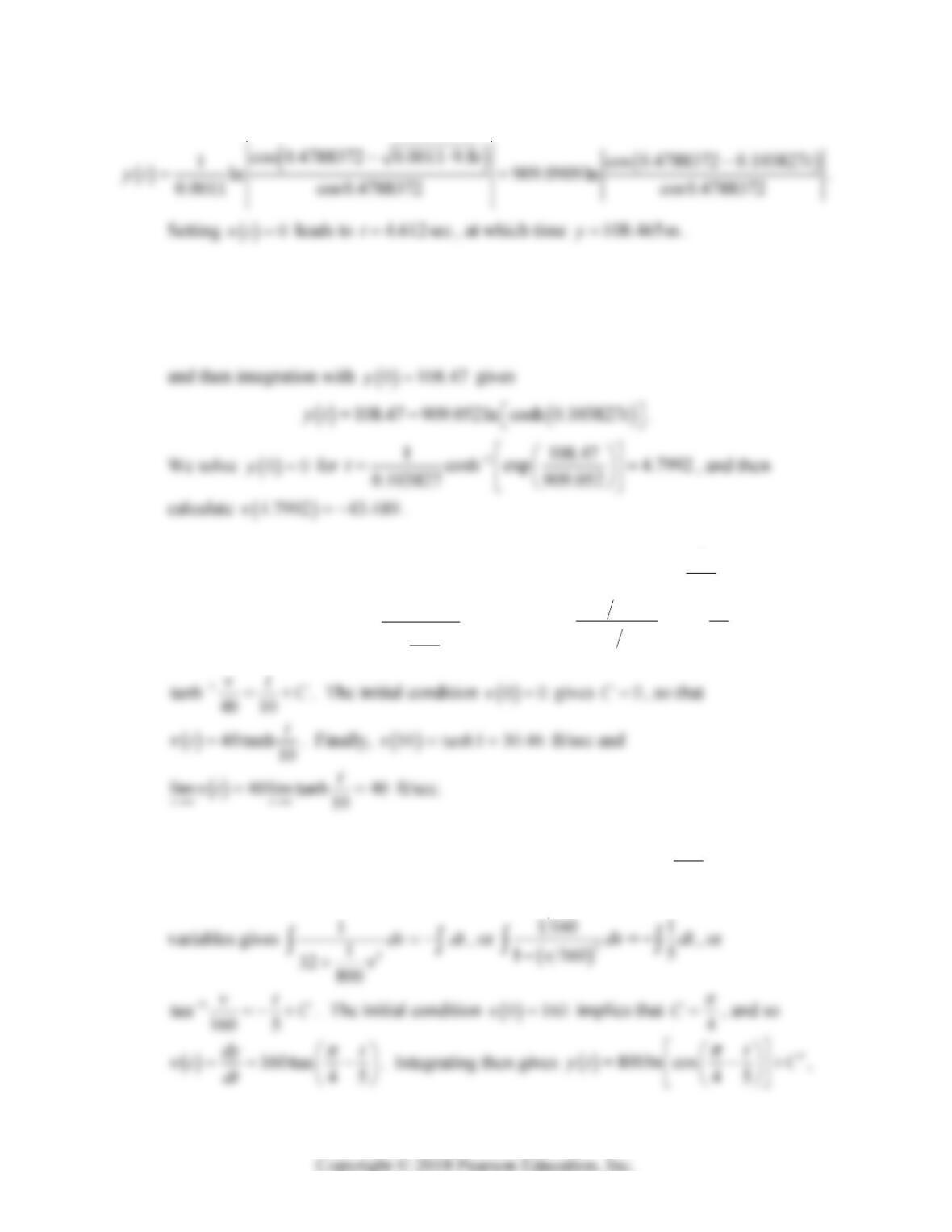
17. Equation (13) from the text gives
11
9.8 tan 0.0011 9.8 94.3880 tan 0.1038267
0.0011
vt C t C t
,
Section 2.3: Acceleration-Velocity Models 133
Then Equation (14) gives
18. We solve the initial value problem 2
9.8 0.0011vv
,
00v much as in Problem
17, except using hyperbolic rather than ordinary trigonometric functions. We first get
94.3841tanh 0.103827vt t ,
19. The initial value problem for the velocity of the motorboat is 2
1
4400
vv
,
00v.
Separating variables gives
2
1
1
4400
dv dt
v
, or
2
140 1
10
140
dv dt
v
, or
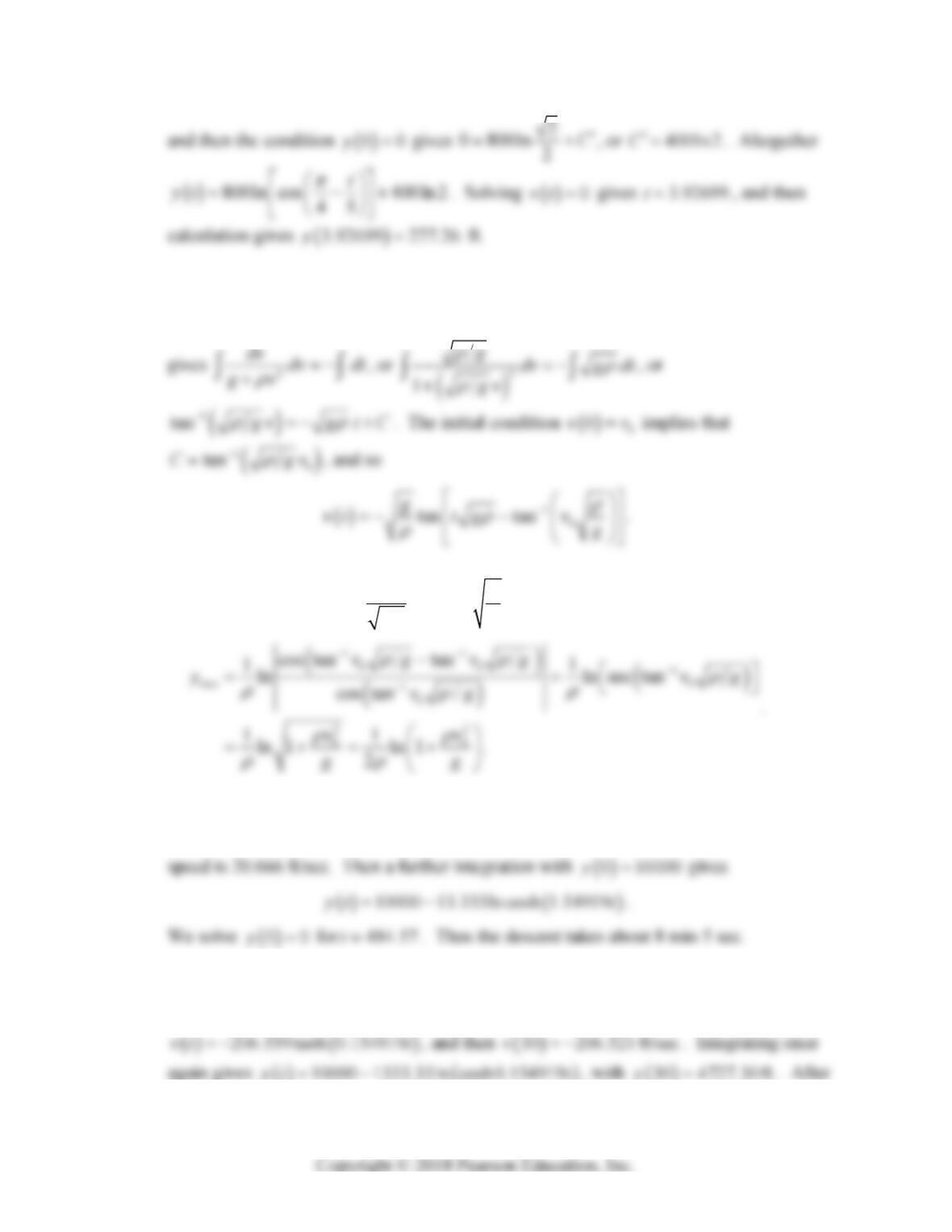
20. The initial value problem for the velocity of the arrow is 2
1
32 800
vv
,
0160v,
with the added condition that
00y, where y is the height of the arrow. Separating
134 Chapter 2: Mathematical Models and Numerical Methods
21. The initial value problem for the velocity of the ball is 2
vgv
,
0
0vv, with the
added condition that
00y, where y is the height of the ball. Separating variables
We solve
0vt for 1
0
1tantv
g
g
and substitute in Equation (17) for
yt:
22. By an integration similar to the one in Problem 19, the solution of the initial value
problem 2
32 0.075vv
,
00v is
20.666 tanh 1.54919vt t , so the terminal
23. Before the parachute opens, the paratrooper’s descent is modeled by the initial value
problem 2
32 0.00075vv
,
00v, with
0 10000y. Solving gives