Section 11.2: Power Series Solutions 615
and the given initial conditions yield 0 011
0and1.cFcF But instead of
proceeding immediately to calculate explicit values of further coefficients, let us first
nn
26. This problem is pretty fully outlined in the textbook. The only hard part is squaring the
power series:
2
27. (b) The roots of the characteristic equation r3 = 1 are r1 = 1, r2 =
=
(1 + i3 )/2, and r3 =
= (1
i 3 )/2. Then the general solution is
() .
x
xx
y
xAeBeCe
(*)
Imposing the initial conditions, we get the equations
SECTION 11.2
POWER SERIES SOLUTIONS
Instead of deriving in detail the recurrence relations and solution series for Problems 1 through
15, we indicate where some of these problems and answers originally came from. Each of the
differential equations in Problems 110 is of the form
616 Chapter 11: Power Series Methods
It yields a solution of the form
y = c0 yeven + c1 yodd
where yeven and yodd denote series with terms of even and odd degrees, respectively. The even-
degree series 24
02 4
ccxcx converges (by the ratio test) provided that
In Problems 1–15 we give first the recurrence relation and the radius of convergence, then the
resulting power series solution.
1. 2024 135
1; ;
;
nn
cc ccc ccc
Section 11.2: Power Series Solutions 617
3. 2;;
(2)
n
n
c
cn
4. 2
41
;
2
nn
n
cc
n
5. 2246
;3; 0
3( 2)
n
n
nc
cccc
n
6. 2
(3)(4)
(1)(2)
nn
nn
cc
nn
The factor ( 3)n in the numerator yields 579 0,ccc and the factor ( 4)n
618 Chapter 11: Power Series Methods
7.
2
2
(4) ;3
3( 1)( )
2
nn
n
cc
nn
The factor ( 4)n yields 6810 0,ccc so yeven is a 4th-degree polynomial.
We find first that 31 51
/ 2 and /120cc cc , and then for 3n that
8. 2
(4)(4)
;2
2( 1)( 2)
nn
nn
cc
nn
We find first that 31 51
5 / 4 and 7 / 32cc cc , and then for 3n that
9. 2
(3)(4) 1
;
(1)(2)
nn
nn
cc
nn
Section 11.2: Power Series Solutions 619
10. 2
(4) ;
3( 1)( 2)
nn
n
cc
nn
The factor (4)n yields 6810 0,ccc so yeven is a 4th-degree polynomial.
We find first that 31 51
/ 6 and / 360cc cc, and then for 3n that
11. 2
2( 5) ;
5( 1)( 2)
nn
n
cc
nn
The factor (5)n yields 7911 0,ccc so yodd is a 5th-degree polynomial.
We find first that 2140 60
, /10 and / 750,cccc cc and then for 4n that
12. 3;
2
n
n
c
cn
When we substitute y = cnxn into the given differential equation, we find first that
20,c so the recurrence relation yields 5811 0ccc also.
620 Chapter 11: Power Series Methods
13. 3;
3
n
n
c
cn
When we substitute y = cnxn into the given differential equation, we find first that
14. 3;
(2)(3)
n
n
c
cnn
When we substitute y = cnxn into the given differential equation, we find first that
20,c so the recurrence relation yields 5811 0ccc also. Then
15. 4;
(3)(4)
n
n
c
cnn
When we substitute y = cnxn into the given differential equation, we find first that
23
0,cc so the recurrence relation yields 610 0cc and 711 0cc also.
Then
16. The recurrence relation is 2
1for 1.
1
nn
n
ccn
n
The factor ( 1)n in the
numerator yields 357 0.ccc When we substitute y = cnxn into the given
Section 11.2: Power Series Solutions 621
Hence
17. The recurrence relation
2
(2)
(1)(2)
n
n
nc
cnn
18. The substitution t = x 1 yields y” + ty’ + y = 0, where primes now denote
differentiation with respect to t. When we substitute y = cntn we get the recurrence
relation
19. The substitution t = x 1 yields (1 – t2)y” – 6ty’ – 4y = 0, where primes now denote
differentiation with respect to t. When we substitute y = cntn we get the recurrence
relation
622 Chapter 11: Power Series Methods
20. The substitution t = x 3 yields (t2 + 1)y” 4ty’ + 6y = 0, where primes now denote
differentiation with respect to t. When we substitute y = cntn we get the recurrence
relation
21. The substitution t = x yields (4t2 + 1)y” = 8y, where primes now denote
differentiation with respect to t. When we substitute y = cntn we get the recurrence
22. The substitution t = x + 3 yields (t2 – 9)y” + 3ty’ 3y = 0, with primes now denoting
differentiation with respect to t. When we substitute y = cntn we get the recurrence
relation
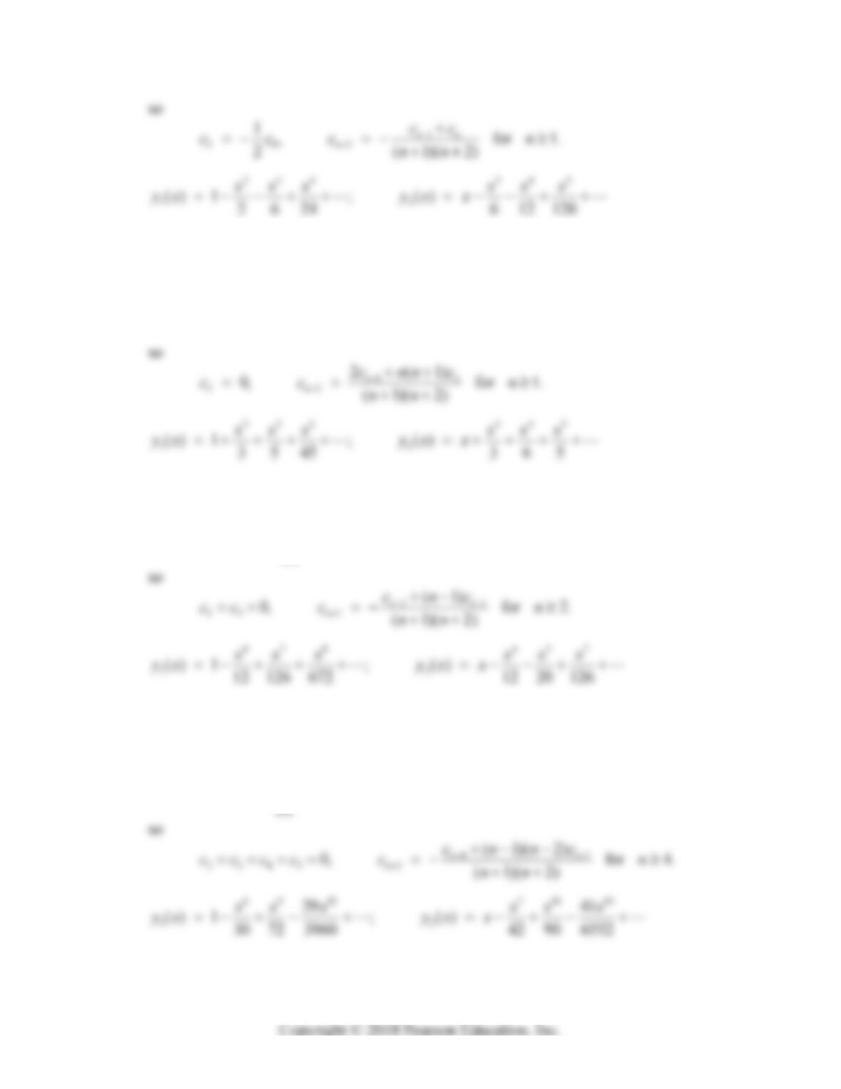
23. Substitution of y = cnxn yields
Section 11.2: Power Series Solutions 623
24. Substitution of y = cnxn yields
21 2
1
22(1)(1)(2) 0,
n
nn n
n
ccnncnncx
25. Substitution of y = cnxn yields
23 2 1 2
2
26 (1) (1)(2) 0,
n
nn n
n
ccx c nc n ncx
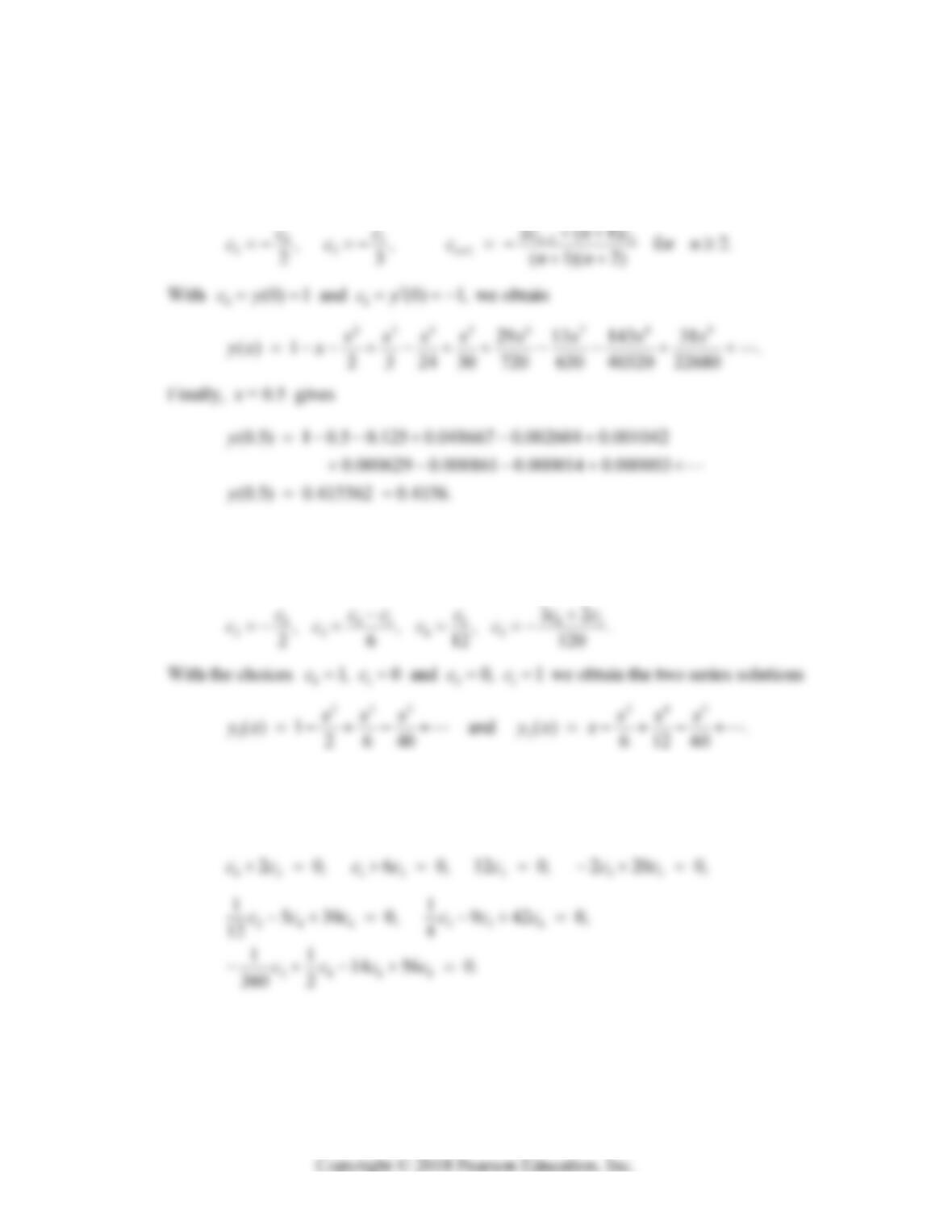
26. Substitution of y = cnxn yields
23
23 4 2 5
412
2 6 12 (2 20 )
( 1)( 2) ( 1)( 2) 0,
n
nnn
ccxcx c cx
cnncnncx
624 Chapter 11: Power Series Methods
27. Substitution of y = cnxn yields
02 13 2 2
2
2(26) 2 (1)(1)(2) 0,
n
nn n
n
cc ccx c ncn ncx
so
28. When we substitute y = cnxn and (1) / !
xnn
exn
and then collect coefficients
of the terms involving 1, x, x2, and x3, we find that
29. When we substitute y = cnxn and 2
cos ( 1) /(2 )!
nn
x
xn
and then collect
coefficients of the terms involving 26
1, , , , ,
x
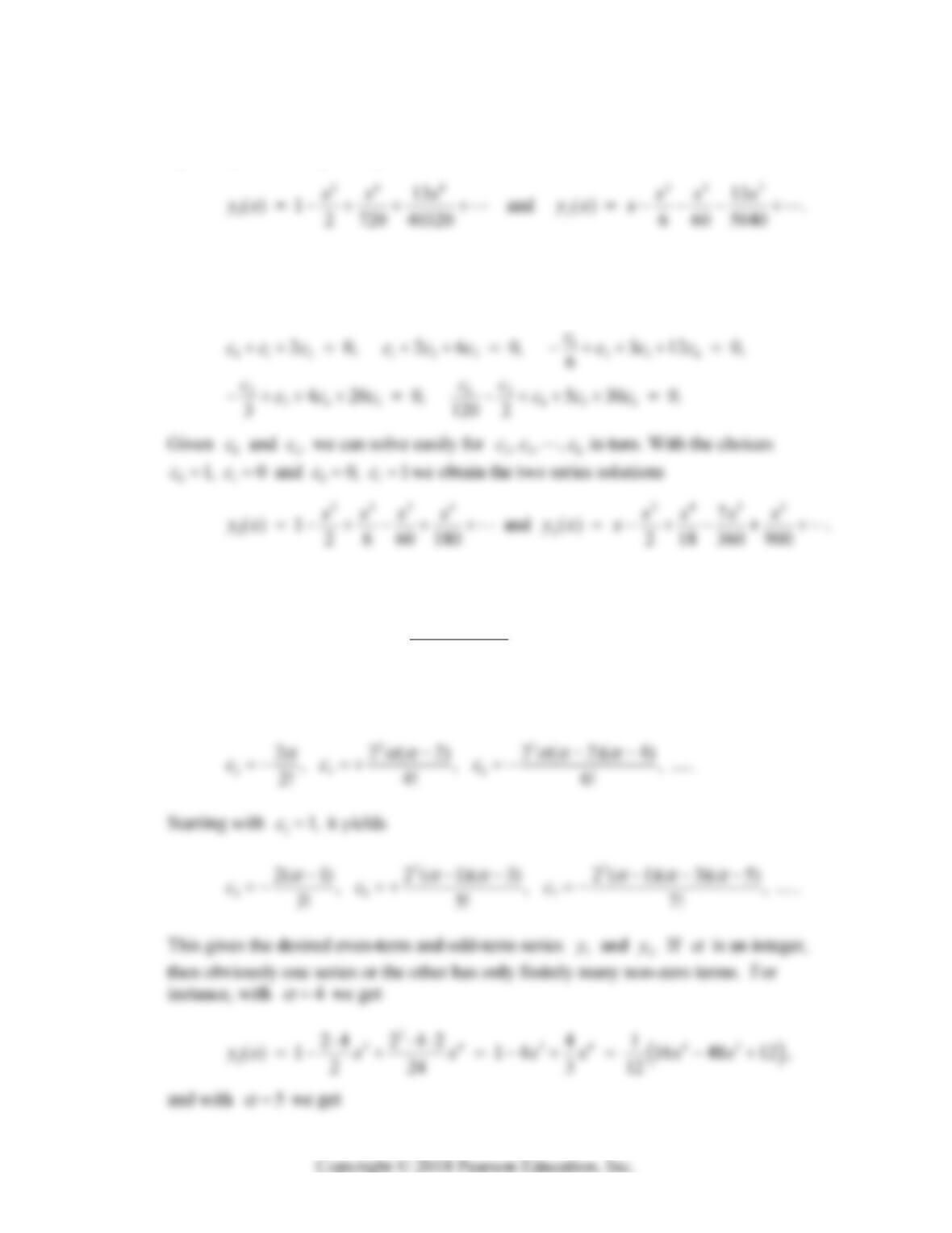
xx we obtain the equations
Section 11.2: Power Series Solutions 625
Given 01
and ,cc we can solve easily for 23 8
,, ,cc c in turn. With the choices
01 0 1
1, 0 and 0, 1cc c c we obtain the two series solutions
30. When we substitute y = cnxn and sin x = (1)nx2n+1 /(2n + 1)!, and then collect
coefficients of the terms involving 25
1,,,,,
x
xx we obtain the equations
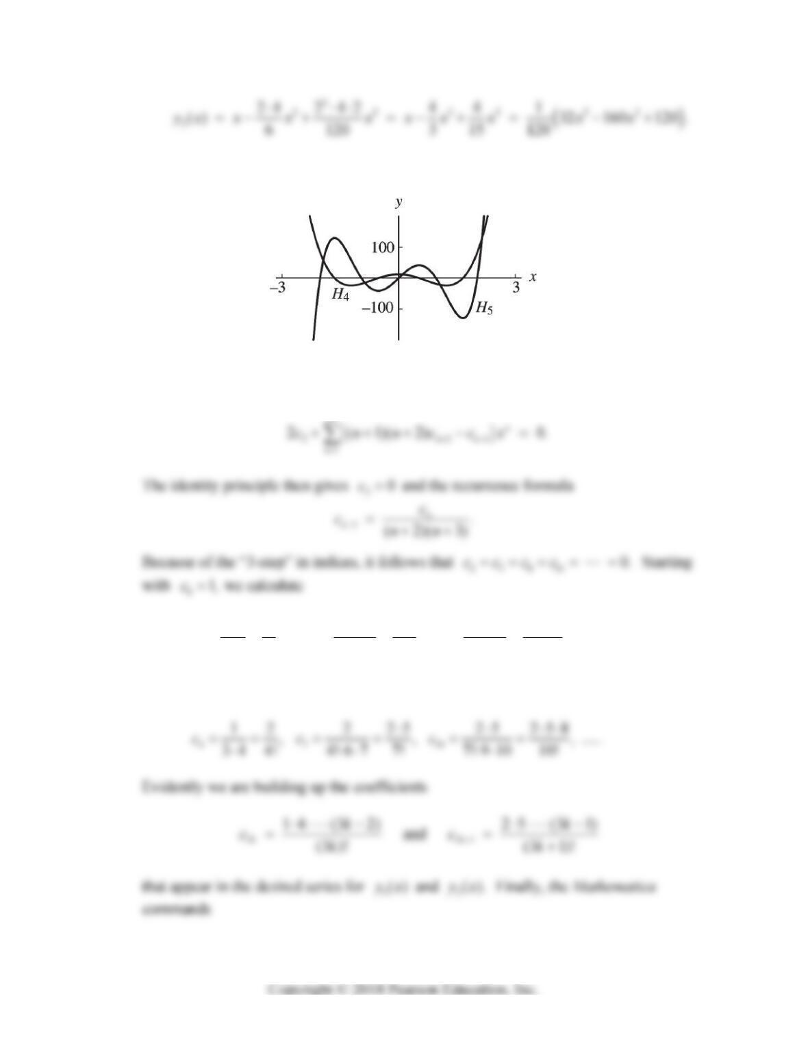
33. Substitution of y = cnxn in Hermite’s equation leads in the usual way to the recurrence
formula
2
2( ) .
(1)(2)
n
n
nc
cnn
Starting with 01,c this formula yields
626 Chapter 11: Power Series Methods
The figure below shows the interlaced zeros of the 4th and 5th Hermite polynomials.
34. Substitution of y = cnxn in the Airy equation leads upon shift of index and collection
of terms to
36 9
11 1 14 14147
,, ,.
2 3 3! 3! 5 6 6! 6! 8 9 9!
cc c
Starting with 11,c we calculate
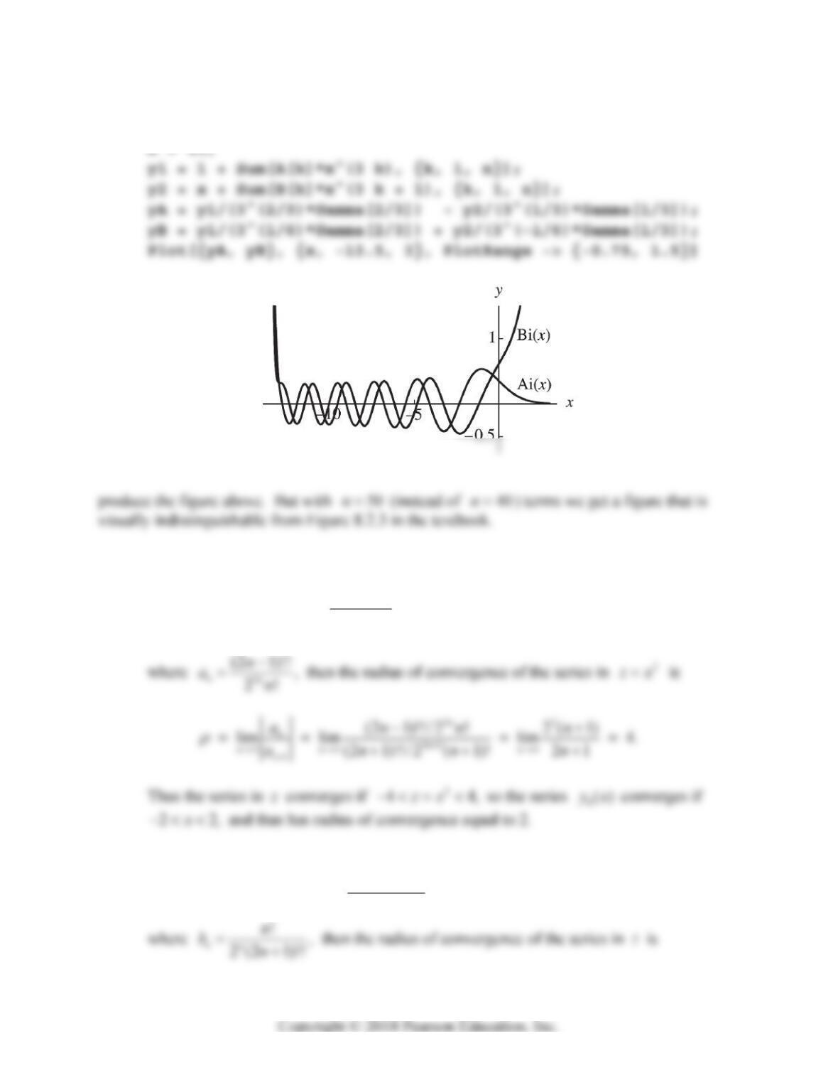
Section 11.2: Power Series Solutions 627
A[1] = 1/6; A[k_] := A[k – 1]/(3 k*(3 k – 1));
B[1] = 1/12; B[k_] := B[k – 1]/(3 k*(3 k + 1));
35. (a) If
2
03
11
(2 1)!!
11
2!
nn
n
n
nn
n
y
xaz
n
y
(b) If
2
1
11
!
11
2(2 1)!!
nn
n
n
nn
n
y
xxxbz
n
628 Chapter 11: Power Series Methods
SECTION 11.3
FROBENIUS SERIES SOLUTIONS
1. Upon division of the given differential equation by x we see that P(x) = 1 x2 and
Q(x) = (sin x)/x. Because both are analytic at x = 0 — in particular, (sin ) / 1xx
as 0x because
2. Division of the differential equation by x yields
10.
x
e
yxy y
x
Because the function
3. When we rewrite the given equation in the standard form of Equation (3) in this section,
we see that p(x) = (cos x)/x and q(x) = x. Because (cos ) /xx as 0
x
it
follows that p(x) is not analytic at x = 0, so x = 0 is an irregular singular point.
Section 11.3: Frobenius Series Solutions 629
5. In the standard form of Equation (3) we have p(x) = 2/(1 + x) and q(x) = 3x2/(1 + x).
Both are analytic x = 0, so x = 0 is a regular singular point. The indicial equation is
6. In the standard form of Equation (3) we have p(x) = 2/(1 x2) and q(x) =
7. In the standard form of Equation (3) we have p(x) = (6 sin x)/x and q(x) = 6, so
x = 0 is a regular singular point with p0 = q0 = 6. The indicial equation is r2 + 5r + 6
9. The only singular point of the differential equation
2
0
11
xx
yyy
xx
is x = 1.
Upon substituting t = x 1, x = t + 1 we get the transformed equation
10. The only singular point of the differential equation 2
21
0
1(1)
yy y
xx
is
x = 1. Upon substituting t = x 1, x = t + 1 we get the transformed equation
11. The only singular points of the differential equation 22
212
0
11
x
yyy
xx
are
630 Chapter 11: Power Series Methods
x = +1: Upon substituting t = x 1, x = t + 1 we get the transformed equation
2( 1) 12 0,
(2) (2)
t
yyy
tt tt
where primes now denote differentiation with respect to
t. In the standard form of Equation (3) we have 2( 1)
() 2
t
pt t
and 12
() .
2
t
qt t
Both these functions are analytic at t = 0, so it follows that x = +1 is a regular singular
12. The only singular point of the differential equation
3
3
30
2(2)
x
yy y
xx
is
x = 2. Upon substituting t = x 2, x = t + 2 we get the transformed equation
13. The only singular points of the differential equation 11
0
22
yyy
xx
are
x = +2 and x = –2.
x = +2: Upon substituting t = x 2, x = t + 2 we get the transformed equation
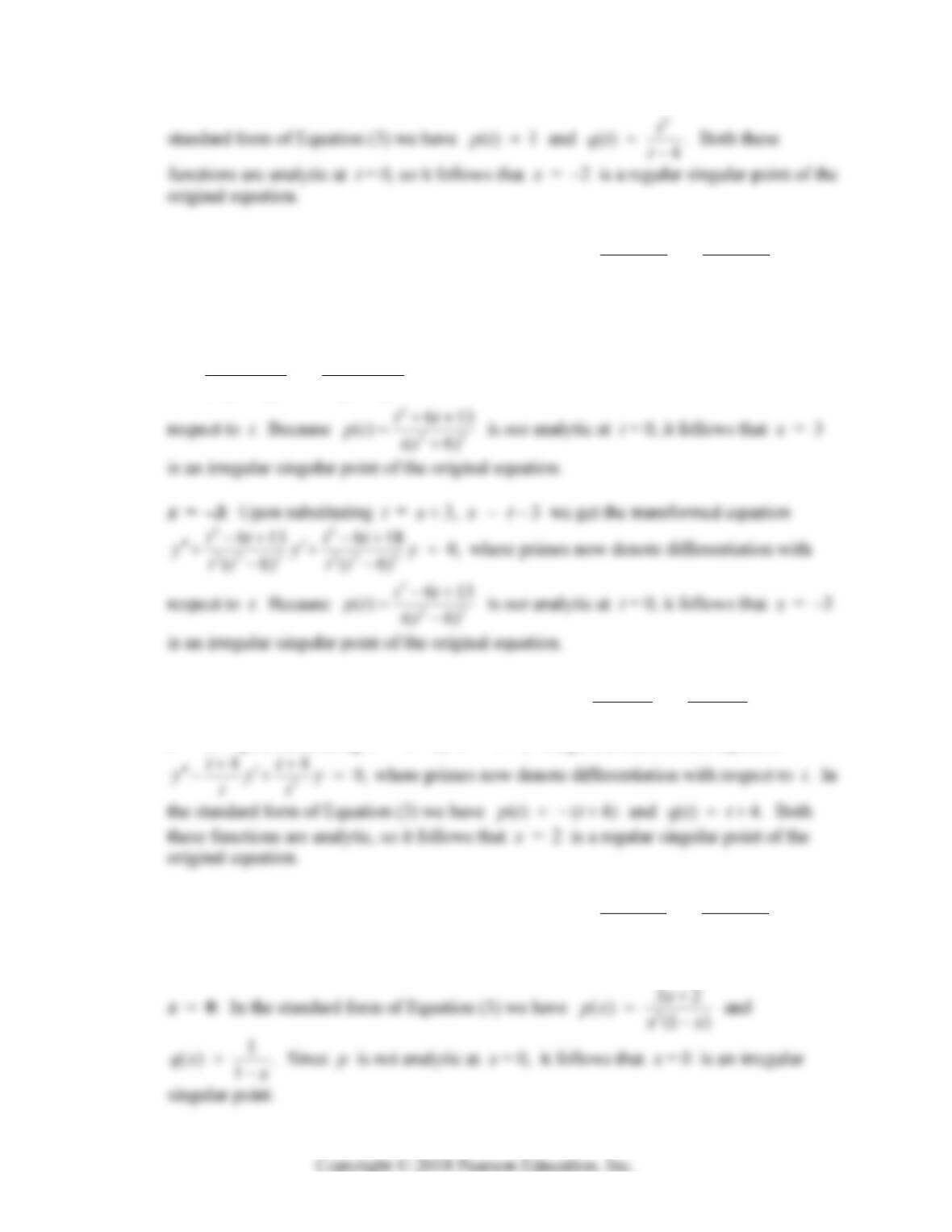
Section 11.3: Frobenius Series Solutions 631
14. The only singular points of the differential equation
22
22 22
94
0
(9) (9)
xx
yyy
xx
are x = +3 and x = –3.
x = +3: Upon substituting t = x 3, x = t + 3 we get the transformed equation
22
22 2 22 2
613 618 0,
(6) (6)
tt tt
yyy
tt tt
where primes now denote differentiation with
15. The only singular point of the differential equation
2
22
42
0
(2) (2)
xx
yyy
xx
is
x = 2. Upon substituting t = x 2, x = t + 2 we get the transformed equation
16. The only singular points of the differential equation 32
32 1 0
(1 ) (1 )
x
yyy
xx xx
are x = 0 and x = 1.
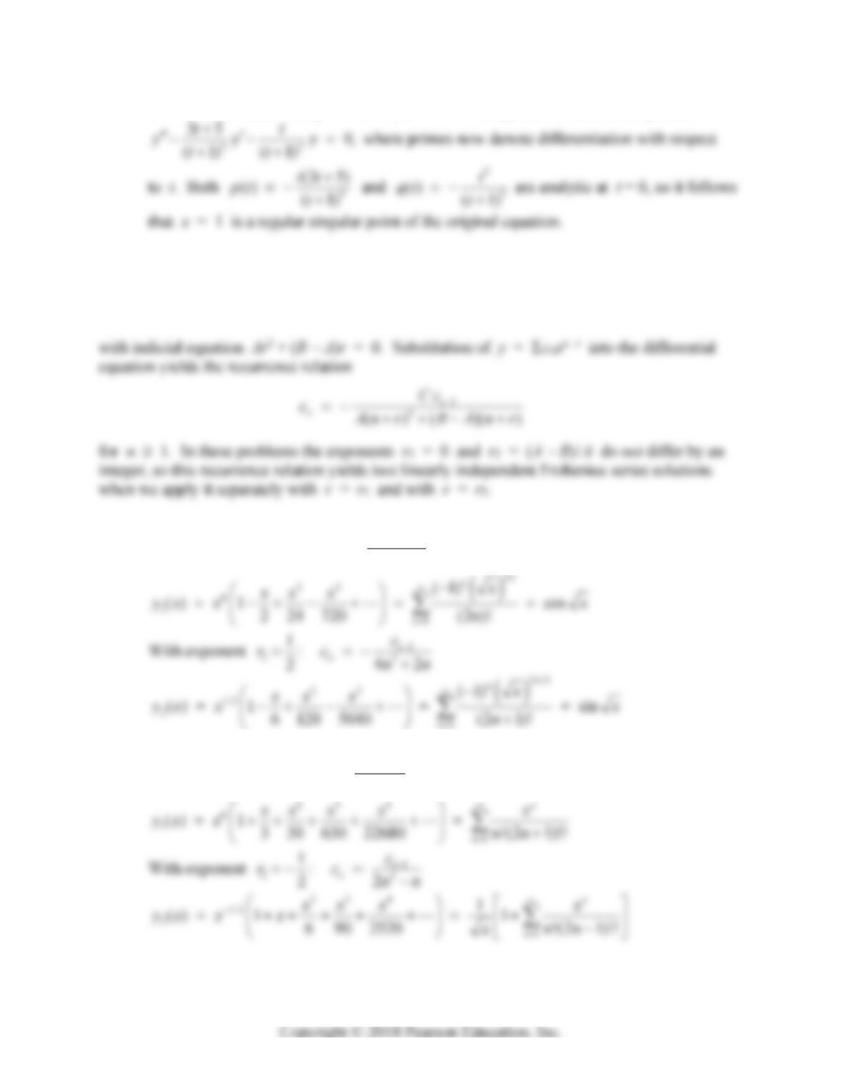
632 Chapter 11: Power Series Methods
x = 1: Upon substituting t = x – 1, x = t + 1 we get the transformed equation
Each of the differential equations in Problems 1720 is of the form
Axy” + By’ + Cy = 0
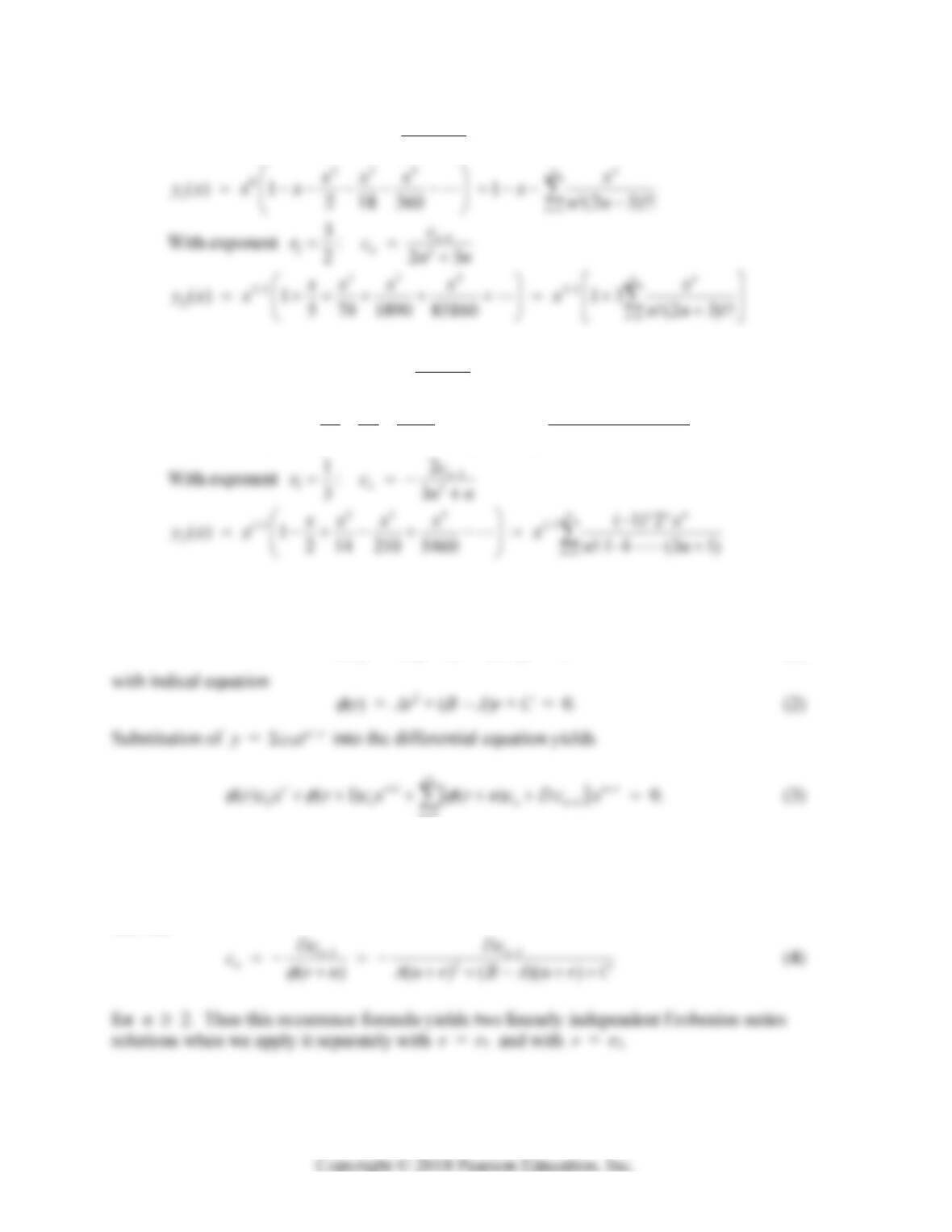
17. With exponent 10:r 1
2
42
n
n
c
cnn
18. With exponent 10:r 1
2
2
n
n
c
cnn
Section 11.3: Frobenius Series Solutions 633
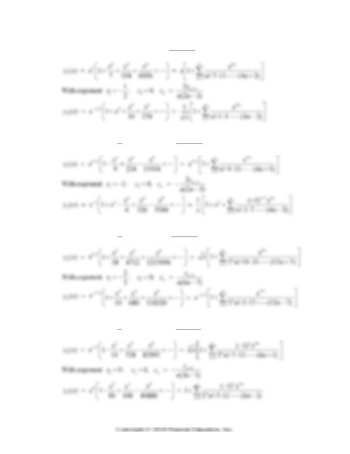
19. With exponent 10:r 1
2
23
n
n
c
cnn
20. With exponent 10:r 1
2
2
3
n
n
c
cnn
23 4
0
1
1
(1)2
() 1 1
5 60 1320 ! 2 5 (3 1)
nnn
n
xx x x
yx x x nn
The differential equations in Problems 21–24 are all of the form
Ax2y” + Bxy’ +(C + Dx2)y = 0 (1)
2
n
In each of Problems 21–24 the exponents r1 and r2 do not differ by an integer. Hence when
we substitute either r = r1 or r = r2 into Equation (*) above, we find that c0 is arbitrary
because ()r
is then zero, that c1 = 0 — because its coefficient (1)r
is then nonzero —
and that
634 Chapter 11: Power Series Methods
21. With exponent 11:r 2
1
2
0, (2 3)
n
n
c
cc
nn
22. With exponent 1
3:
2
r 2
1
2
0, (2 5)
n
n
c
ccnn
23. With exponent 1
1:
2
r 2
10, (6 7)
n
n
c
cc
nn
24. With exponent 1
1:
3
r 2
10, (3 1)
n
n
c
ccnn