Section 10.5: Periodic and Piecewise Continuous Input Functions 595
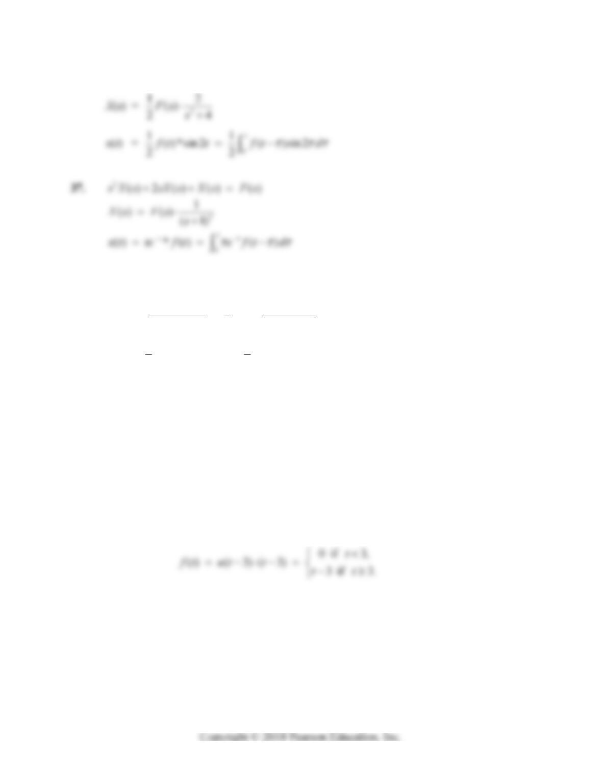
36. s2X(s) + 4X(s) = F(s)
f
38. 2() 4 () 13 () ()sXs sXs Xs Fs
22
() 1 3
() ()
413 3 (2)9
Fs
Xs Fs
ss s
22
0
11
() ()* sin3 sin3
33
t
t
x
tftet eft d
SECTION 10.5
PERIODIC AND PIECEWISE CONTINUOUS
INPUT FUNCTIONS
In Problems 1 through 10, we first derive the inverse Laplace transform ( ) of ( )
f
tFs and then
show the graph of ( ).
f
t
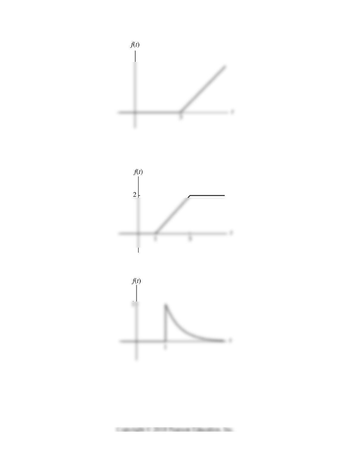
1.
3
() s
Fs e t
L so Eq. (3b) in Theorem 1 gives
596 Chapter 10: Laplace Transform Methods
2.
0if 1,
() ( 1)( 1) ( 3)( 3) 1if1 3,
2if 3.
t
ft t ut t ut t t
t
3.
2
()
s
t
Fs e e
L so 2( 1)
2( 1)
0if 1,
() ( 1) if 1.
t
t
t
ft ut e et
Section 10.5: Periodic and Piecewise Continuous Input Functions 597
4. 22
() {} {}
ss
Fs e t ee t
LLso
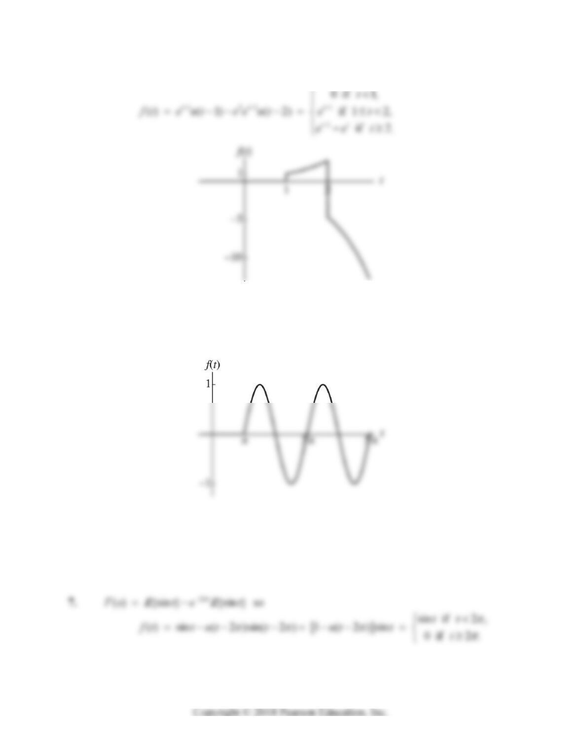
5. () {sin}
s
Fs e t
L so
0if ,
() ( ) sin( ) ( )sin sin if .
t
ft ut t ut t tt
6. () {cos}
s
Fs e t
L so
0if 1,
() ( 1) cos ( 1) ( 1)cos cos if 1.
t
ft ut t ut t tt
598 Chapter 10: Laplace Transform Methods
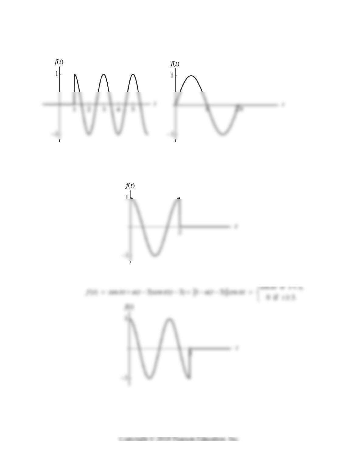
The left-hand figure below is the graph for Problem 6 on the preceding page, and the right-hand
figure is the graph for Problem 7.
8. 2
() {cos } {cos }
s
Fs t e t
LL so
cos if 2,
( ) cos ( 2) cos ( 2) 1 ( 2) cos 0if 2.
tt
ft t ut t ut t t
9. 3
() {cos } {cos }
s
Fs t e t
LL so
Section 10.5: Periodic and Piecewise Continuous Input Functions 599
10. 2
() {2cos2} {2cos2}
ss
Fs e t e t
LL so
( ) 2 ( )cos2( ) 2 ( 2 )cos2( 2 )
ft ut t ut t
11.
33
222
() 2 ( 3) 2 so ( ) 1 .
ss
ft ut Fs e e
sss
12.
3
3
1
() ( 1) ( 4) so ( ) .
ss
ss
ee
f t ut ut Fs e e
ss s
s
15. () [1(3)]sin sin (3)]sin(3)soft ut t t ut t
33
22 2
11
() .
11 1
s
s
ee
Fs ss s
600 Chapter 10: Laplace Transform Methods
17. ( ) [ ( 2) ( 3)]sin ( 2)sin ( 2) ( 3)sin ( 3) sof t ut ut t ut t ut t
18. ( ) [ ( 3) ( 5)]cos ( 3) sin ( 3) ( 5) sin ( 5) so
22 2
t
f t ut ut ut t ut t
19. If () 1then() (1) (1)(1)sogt t f t ut t ut gt
22
11 (1)
() () { 1} .
s
ss s es
Fs e Gs e Lt e ss s
21. If() 1and() 2gt t ht t then
22. f(t) = [u1(t) – u2(t)] t3 = u1(t)g(t – 1) – u2(t)h(t – 2) where
23. With ( ) 1 and 1ft p, Formula (6) in the text gives
1
t
Section 10.5: Periodic and Piecewise Continuous Input Functions 601
24. With f(t) = cos kt and p = 2
/k, Formula (6) and the integral formula
25. With p = 2a and f(t) = 1 if 0 t a, f(t) = 0 if a < t 2a, Formula (6) gives
26. With p = a and f(t) = t/a, Formula (6) and the integral formula ( 1)
uu
ue du u e
(with ust ) give
27. G(s) =
/()ta ftL = (1/as2) – F(s). Now substitution of the result of Problem 26
in place of F(s) immediately gives the desired transform.
28. This computation is very similar to the one in Problem 26, except that p = 2a:
602 Chapter 10: Laplace Transform Methods
29. With p = 2
/k and f(t) = sin kt for 0 t
/k while f(t) = 0 for
/k t 2
/k,
Formula (6) and the integral formula
22
sin cos
sin
at at abtb bt
ebtdte C
ab
give
30. ()()()()(/)(/),ht ft gt ft ut kft k
so Problem 29 gives
s
s
//
() () () 1 ()
sk sk
Hs Fs e Fs e Fs
In Problems 31–42, we first write and transform the appropriate differential equation. Then we
solve for the transform of the solution, and finally inverse transform to find the desired solution.
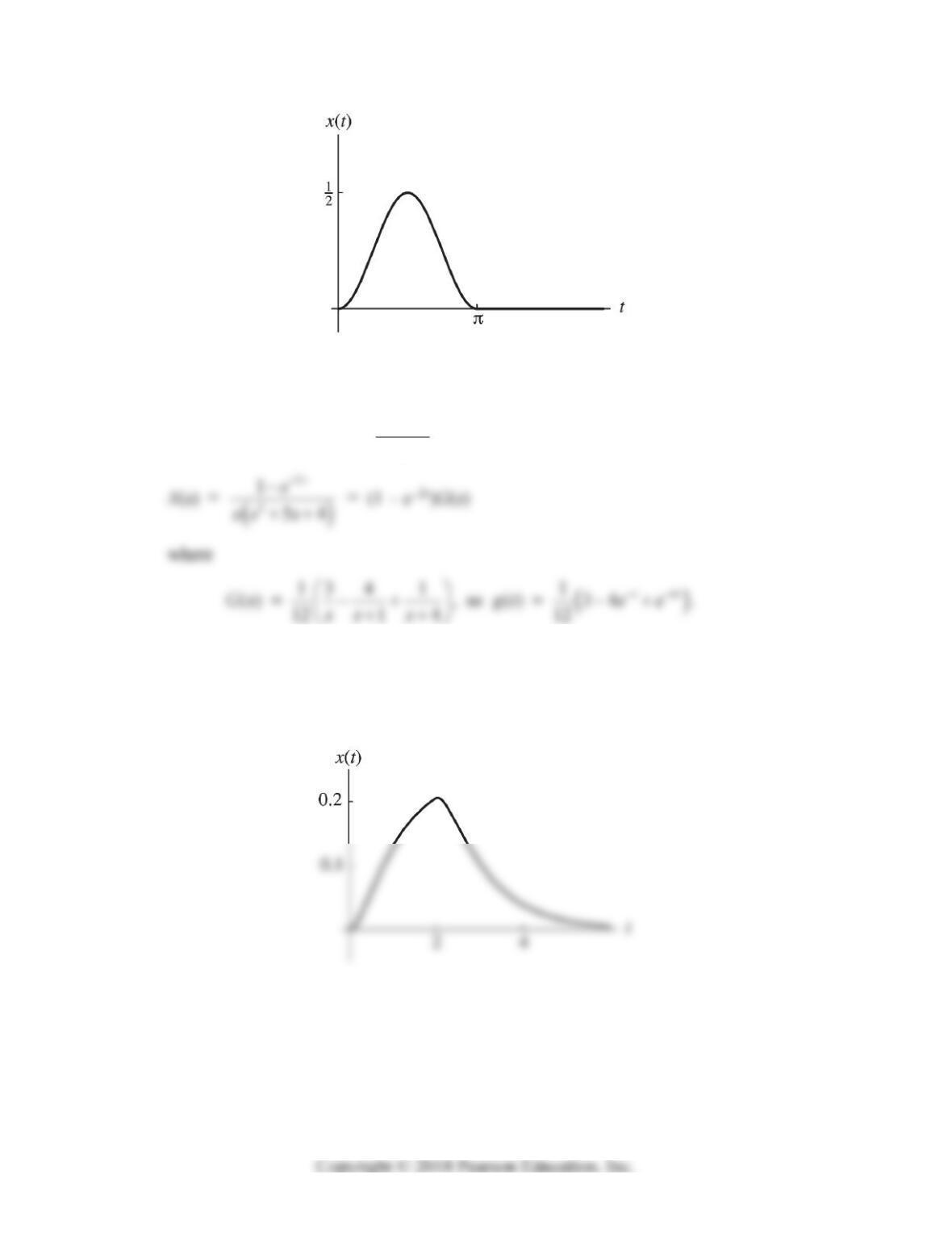
31. x” + 4x = 1 – u(t –
)
s2X(s) + 4X(s) = 1
s
e
s
Section 10.5: Periodic and Piecewise Continuous Input Functions 603
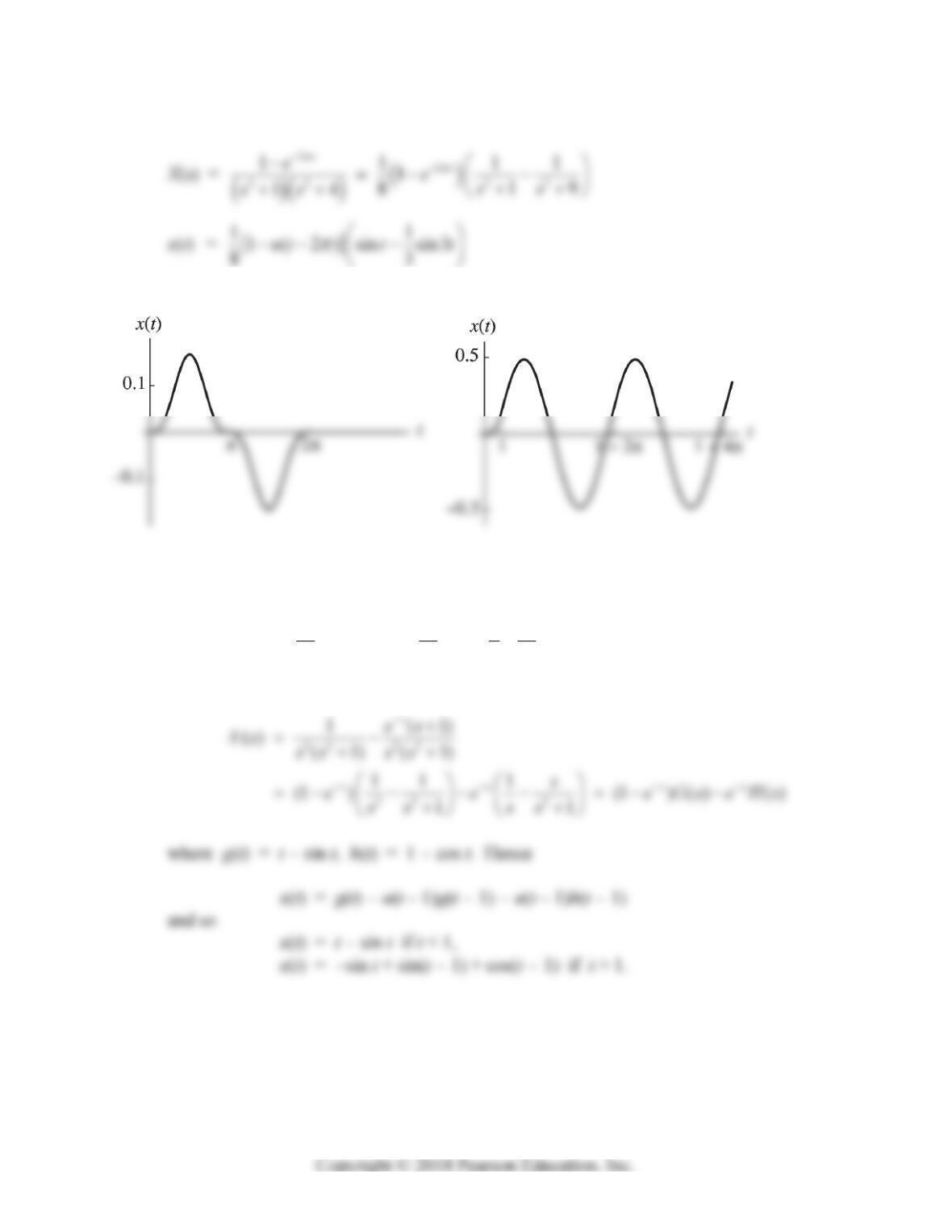
32. x” + 5x’ + 4x = 1 – u(t – 2)
s2X(s) + 5s X(s) + 4X(s) =
2
1
s
e
s
It follows that
() if 2,
() () ( 2) ( 2) () ( 2) if 2.
gt t
xt gt ut gt gt gt t
604 Chapter 10: Laplace Transform Methods
33. x” + 9x = [1 – u(t – 2
)]sin t
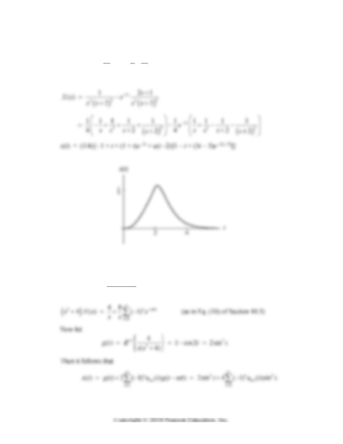
The left-hand figure below show the graph of this position function.
34. x” + x = [1 – u(t – 1)] t 1 ( 1) ( 1), where ( ) 1ut ft ft t
s2X(s) + X(s) = 222
1111
()
ss
eGs e
ssss
It follows that
The right-hand figure above shows the graph of this position function.
Section 10.5: Periodic and Piecewise Continuous Input Functions 605
35. x + 4x + 4x = [1 – u(t – 2)]t = t – u(t – 2)g(t – 2) where () 2gt t
(s + 2)2X(s) = 2
22
121
s
e
sss
36. x” + 4x = f(t), x(0) = x’(0) = 0
241
4() 1
s
s
e
sXs
se
(by Example 5 of Section 10.5)
606 Chapter 10: Laplace Transform Methods
Hence
Consequently the complete solution
() 2sin sin
x
ttt
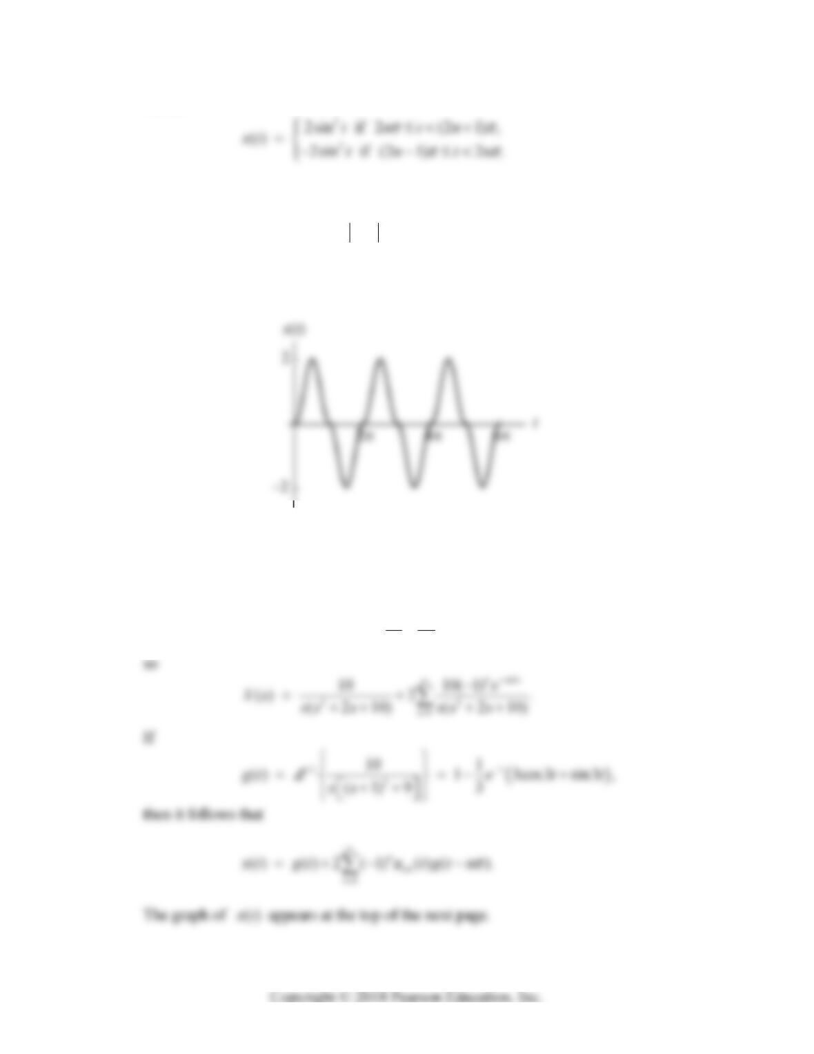
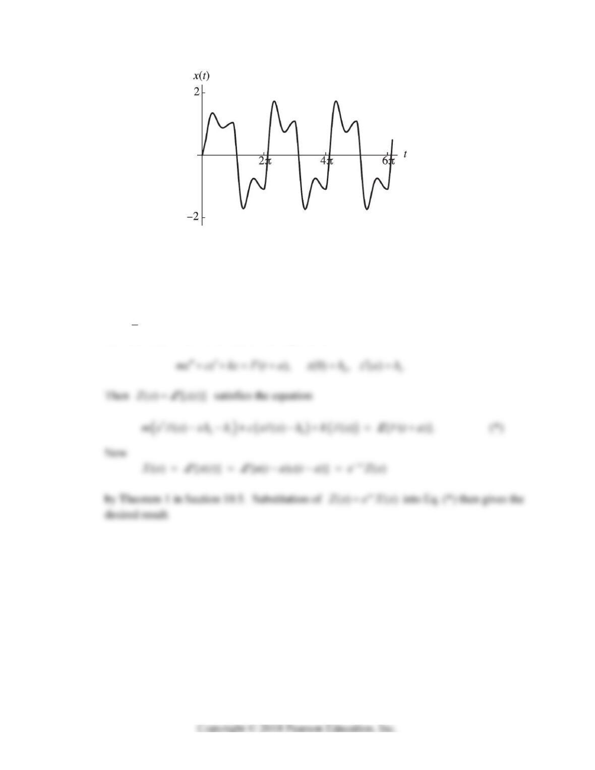
is periodic, so the transient solution is zero. The graph of ():
x
t
37. x” + 2x’ + 10x = f(t), x(0) = x’(0) = 0
As in the solution of Example 7 we find first that
2
1
10 20
210() (1) ,
nns
n
ss Xs e
ss
x
Section 10.5: Periodic and Piecewise Continuous Input Functions 607
38. If the function ()
x
t satisfies the initial value problem
01
(), ( ) , ( )mx cx kx F t x a b x a b
for
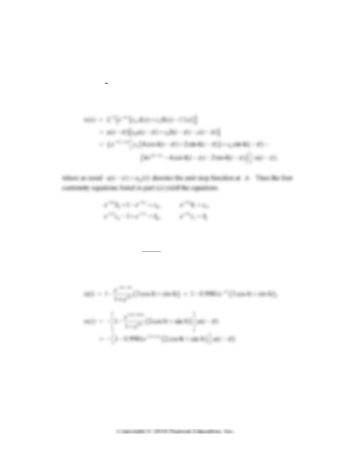
ta and () 0xt for ,ta then we may write () ( ) ( )
x
tutazta
where the
function ()zt satisfies the initial value problem
Z
608 Chapter 10: Laplace Transform Methods
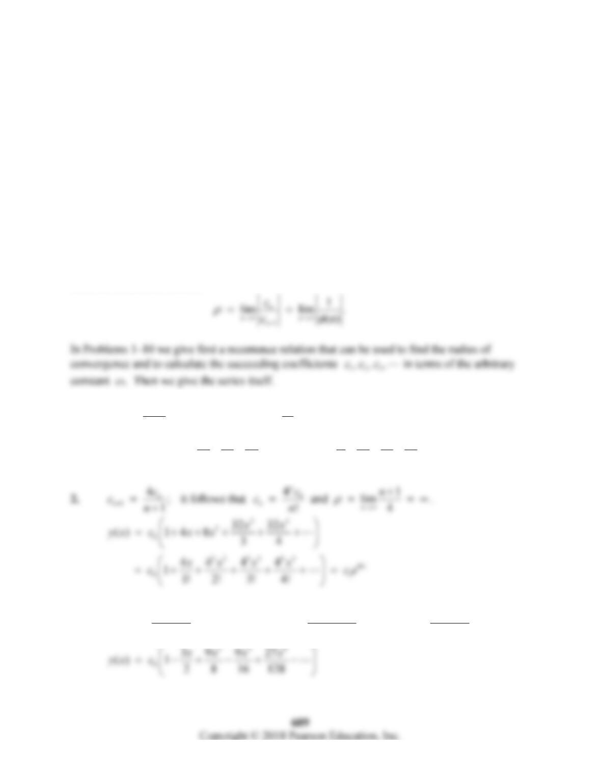
39. When we substitute the inverse Laplace transforms ( ), ( ), ( )at bt ct given at the
beginning of part (c), we get
01
2
1
01
4
() () () ()
4cos4 2sin4 sin4 4 4cos4 2sin4 .
t
vt bat bbt ct
eb t tb t t t
Similarly, Theorem 1 in this section gives
that we solve readily for
2
00 11
2
10.996372, 0.
1
e
bc bc
e
Finally, these values for the coefficients yield
CHAPTER 11
POWER SERIES METHODS
SECTION 11.1
INTRODUCTION AND REVIEW OF POWER SERIES
The power series method consists of substituting a series y = cnxn into a given differential
equation in order to determine what the coefficients {cn} must be in order that the power series
will satisfy the equation. It might be pointed out that, if we find a recurrence relation in the form
cn+1 =
(n)cn, then we can determine the radius of convergence
of the series solution directly
from the recurrence relation
1. 1;
1
n
n
c
cn
it follows that 0and lim ( 1)
!
nn
c
cn
n
.
234 234
00 0
() 1 1
2624 1!2!3!4!
x
xxx xxxx
yx c x c ce
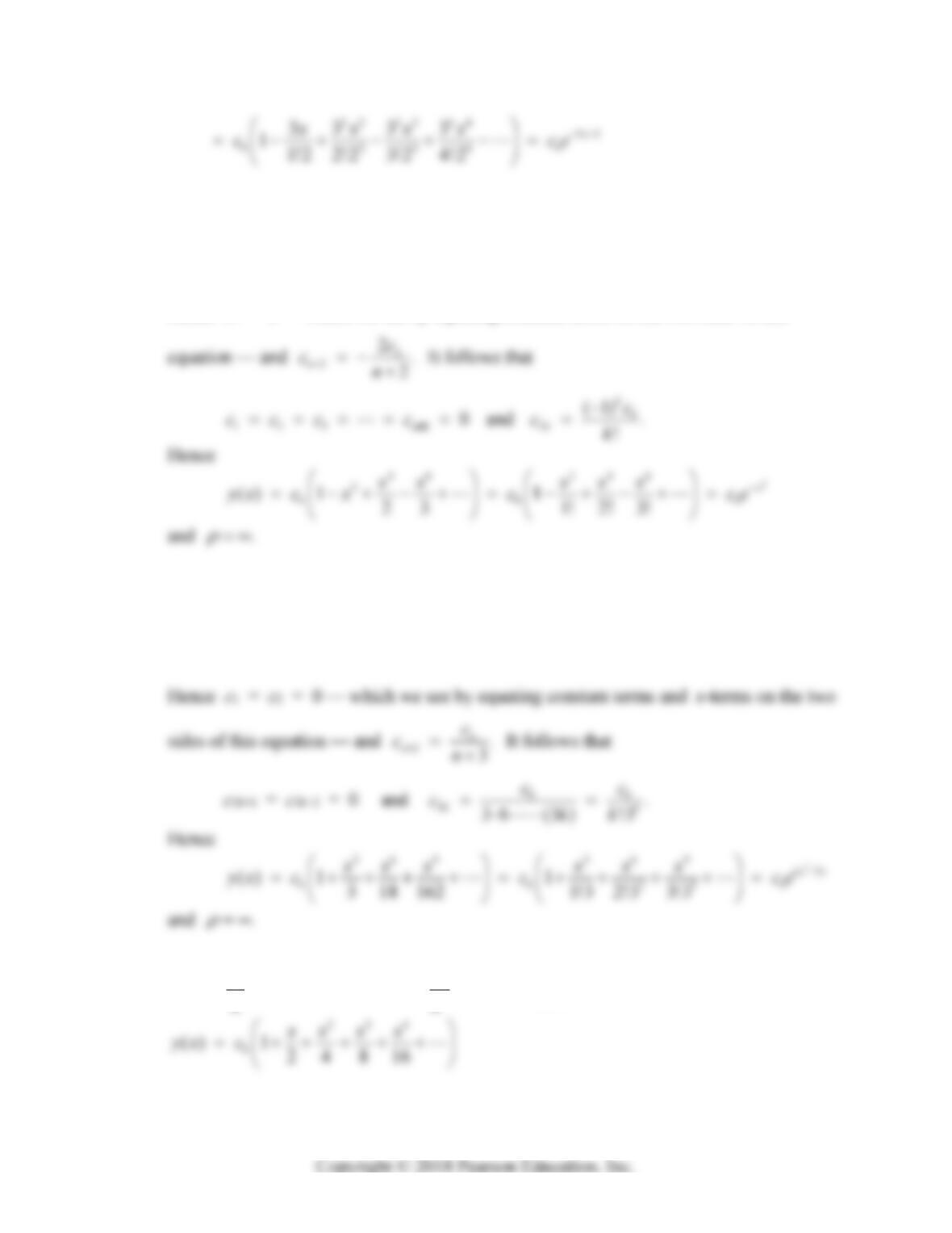
3.
1
3;
21
n
n
c
cn
it follows that
0
13 2 1
and lim
2! 3
nn
nnn
cn
cn
.
610 Chapter 11: Power Series Methods
4. When we substitute y = cnxn into the equation y’ + 2xy = 0, we find that
1
12
0
(2) 2 0.
n
nn
n
cnccx
Hence c1 = 0 — which we see by equating constant terms on the two sides of this
5. When we substitute y = cnxn into the equation 2,
y
xy
we find that
2
12 3
0
2(3) 0.
n
nn
n
ccx nc cx
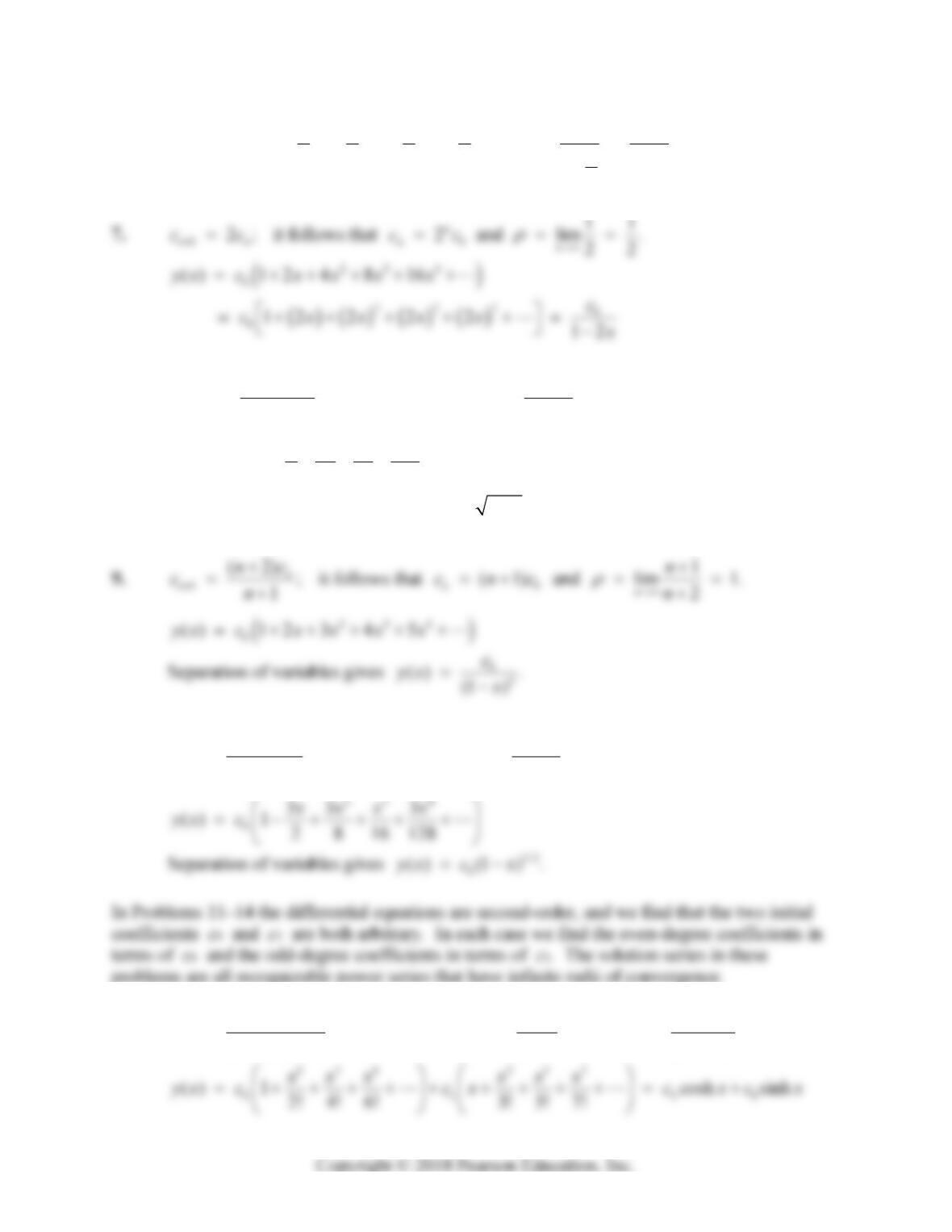
6. 1;
2
n
n
c
c it follows that 0and lim 2 2.
2
nnn
c
c
Section 11.1: Introduction and Review of Power Series 611
234
00
0
2
122 2 2 2
12
x
xxx c c
cx
x
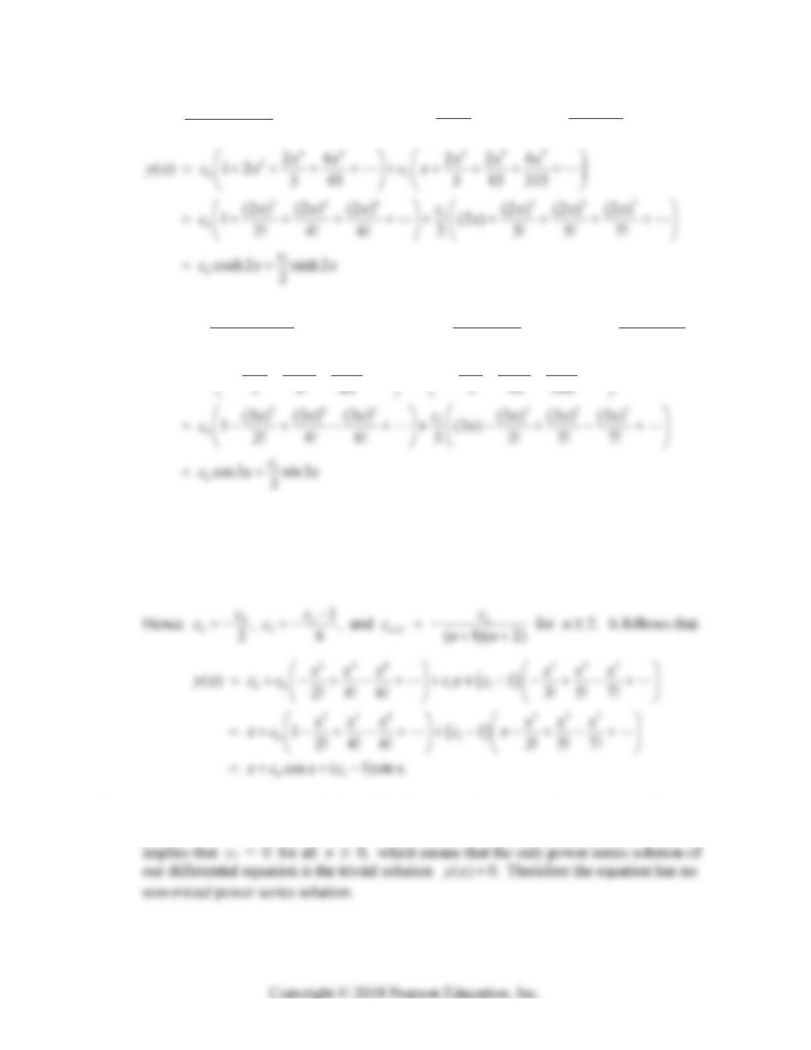
8. 1
(2 1) ;
22
n
n
nc
cn
it follows that 22
lim 1.
21
n
n
n
23 4
0
5
() 1 2 8 16 128
xx x x
yx c
Separation of variables gives 0
() 1 .yx c x
10. 1
(2 3) ;
22
n
n
nc
cn
it follows that 22
lim 1.
23
n
n
n
11. 1;
(1)(2)
n
n
c
cnn
it follows that 0
2(2 )!
k
c
ck
and 1
21 .
(2 1)!
k
c
ck
612 Chapter 11: Power Series Methods
12.
2
4;
12
n
n
c
cnn
it follows that
2
0
2
2
(2 )!
k
k
c
ck
and
2
1
21
2.
(2 1)!
k
k
c
ck
13.
2
9;
(1)(2)
n
n
c
cnn
it follows that
2
0
2
(1)3
(2 )!
kk
k
c
ck
and
2
1
21
(1)3 .
(2 1)!
kk
k
c
ck
246 357
01
9 27 81 3 27 81
() 1 2 8 80 2 40 560
xxx xxx
yx c c x
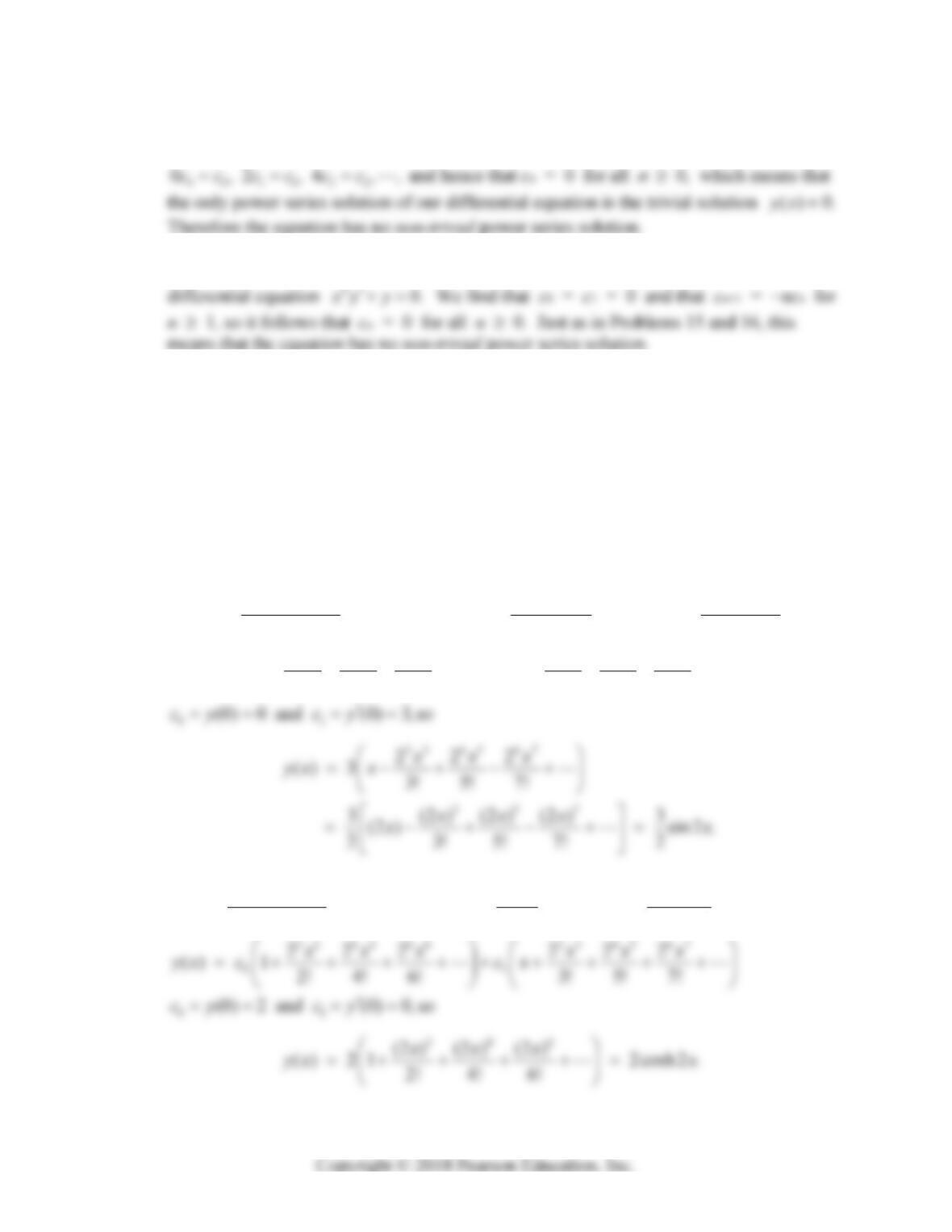
14. When we substitute y = cnxn into y” + y x = 0 and split off the terms of degrees 0
and 1, we get
(2c2 + c0) + (6c3 + c1 1) x + 2
2
[( 1)( 2) ] = 0.
n
nn
n
nnccx
15. Assuming a power series solution of the form y = cnxn, we substitute it into the
differential equation 0xy y
and find that (n + 1)cn = 0 for all n 0. This
Section 11.1: Introduction and Review of Power Series 613
16. Assuming a power series solution of the form y = cnxn, we substitute it into the
differential equation 2
x
yy
and find that 2 nn
nc c for all n 0. This implies that
17. Assuming a power series solution of the form y = cnxn, we substitute it into the
18. When we substitute and assumed power series solution y = cnxn into x3y’ = 2y, we
find that c0 = c1 = c2 = 0 and that cn+2 = ncn/2 for n 1. Hence cn = 0 for all
n 0, just as in Problems 15–17.
In Problems 19–22 we first give the recurrence relation that results upon substitution of an
assumed power series solution y = cnxn into the given second-order differential equation.
Then we give the resulting general solution, and finally apply the initial conditions 0
(0)
y
c
and 1
(0)
y
c
to determine the desired particular solution.
19.
222
01
2221
2 ( 1) 2 ( 1) 2
for 0, so and .
( 1)( 2) (2 )! (2 1)!
kk kk
n
nkk
ccc
cncc
nn k k
22 44 66 23 45 67
01
222 222
() 1 2! 4! 6! 3! 5! 7!
xxx xxx
yx c c x
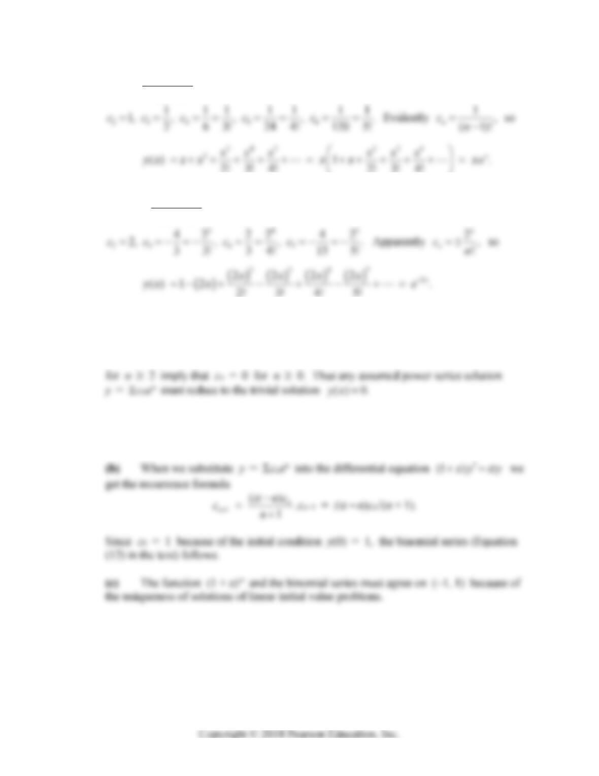
20.
222
01
2221
222
for 0, so and .
( 1)( 2) (2 )! (2 1)!
kk
n
nkk
ccc
cncc
nn k k
614 Chapter 11: Power Series Methods
21. 1
101
2for 1; with (0) 0 and (0) 1,
(1)
nn
n
nc c
cncycy
nn
we obtain
2! 3! 4! 2! 3! 4!
22. 1
101
2for 1; with (0) 1 and (0) 2,
(1)
nn
n
nc c
cncycy
nn
we obtain
23. c0 = c1 = 0 and the recursion relation
(n2 n + 1)cn + (n 1)cn1 = 0
24. (a) The fact that ( )
y
x = (1 + x)
satisfies the differential equation
(1)
x
yy
follows immediately from the fact that 1
() (1 ) .yx x
x
25. Substitution of 0
n
n
ncx
into the differential equation
y
yy
leads routinely —
via shifts of summation to exhibit n
x
-terms throughout — to the recurrence formula
21
(2)(1) (1) ,
nnn
nnc ncc