Section 8.3: Spectral Decomposition Methods 495
15. 12
75
;54, 54
43 ii
A
16. 12
50 20 ; 100, 10
100 60
A
42 52
11 1 1
In Problems 17, 18, and 20 the coefficient matrix A is 33 with distinct eigenvalues 123
,,.
Looking at Equations (7) and (3) in Section 8.3, we see that
3
12
123
t
tt
t
eee e
APPP
(3)
17. 123
414
171; 0, 6, 9
414
A
496 Chapter 8: Matrix Exponential Methods
1
10 1
11
6 9 000
54 2 10 1
PAIAI
18. 123
122
271; 0, 6, 9
217
A
1
16 4 4
11
69 411
54 18 41 1
PAIAI
Section 8.3: Spectral Decomposition Methods 497
19. 123
411
141; 6, 3, 3
114
A
Here we have the eigenvalue 16
of multiplicity 1 and the eigenvalue 23
of
multiplicity 2. By Example 2 in Section 8.3, the desired matrix exponential is given by
so 12
() 1/9and () /9aa
in the notation of Equation (25) in the text. Therefore
Equation (26) there gives
2
2
11 2
111
11
()( ) 3 111,
93
111
a
PAAI AI
20. 123
513
1 7 1 ; 2, 6, 9
315
A
498 Chapter 8: Matrix Exponential Methods
2
121
11
29 242
12 6 121
PAIAI
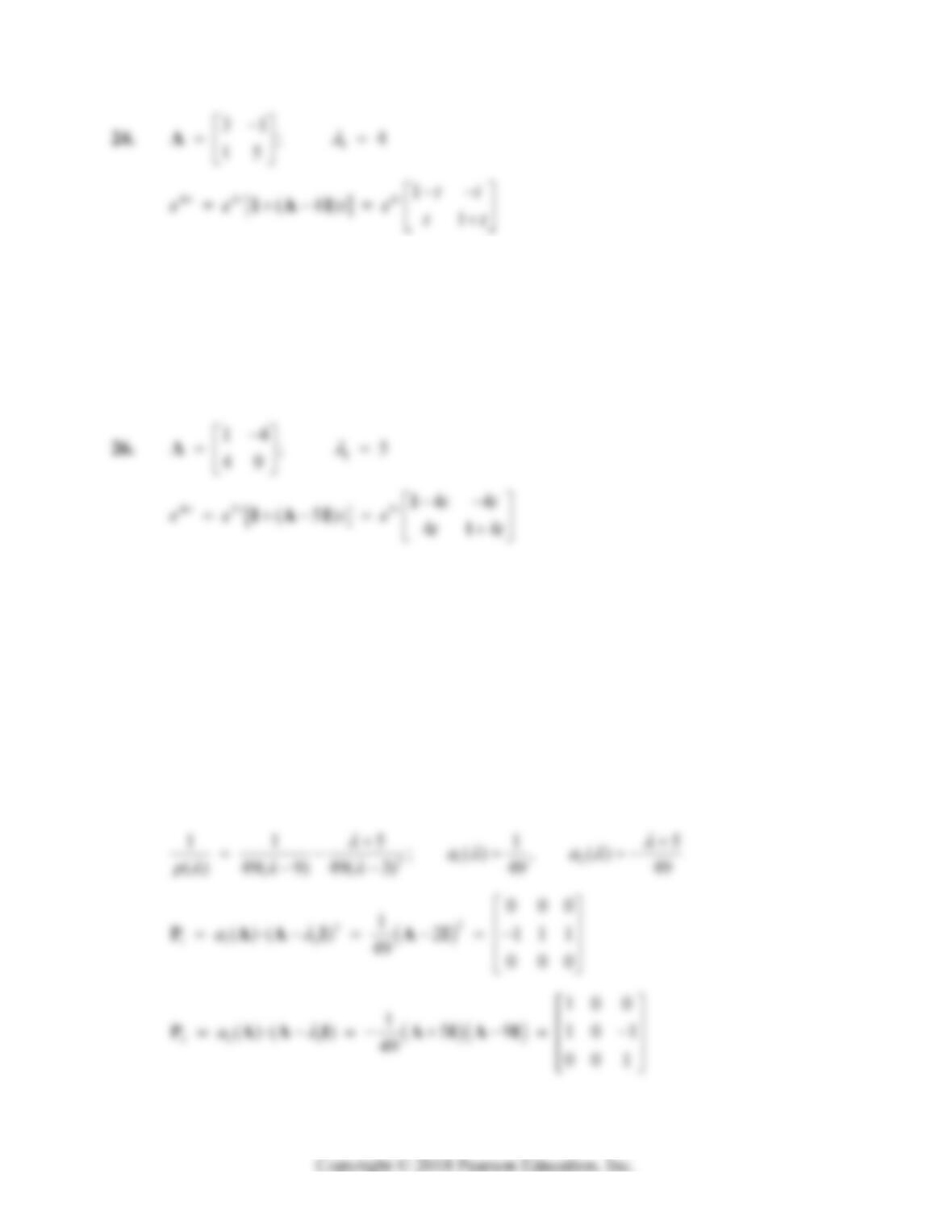
In Problems 21–30 here we want to use projection matrices to find fundamental matrix solutions
of the linear systems given in Problems 1–10 of Section 7.6. In each of Problems 21–26, the
22coefficient matrix A has characteristic polynomial of the form 2
1
() ( )p
and thus a
single eigenvalue 1
of multiplicity 2. Consequently, Example 5 in Section 8.3 gives the
desired fundamental matrix
1
1
().
t
t
ee t
AIA I (6)
21. 1
21
;3
14
A
33
1
(3) 1
tt t
tt
ee tett
AIA I
Section 8.3: Spectral Decomposition Methods 499
25. 1
71
;5
43
A
55
12
(5) 412
tt t
tt
ee te tt
AIA I
Each of the 33 coefficient matrices in Problems 27–30 has a characteristic polynomial of the
form 2
12
() ( )(( )p
yielding an eigenvalue 1
of multiplicity 1 and an eigenvalue
2
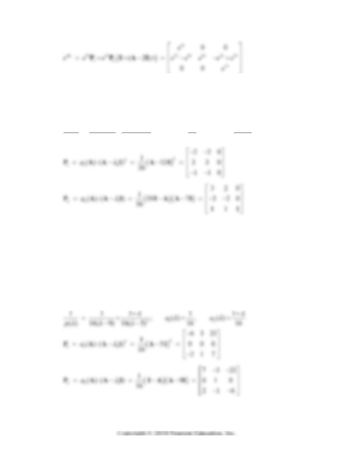
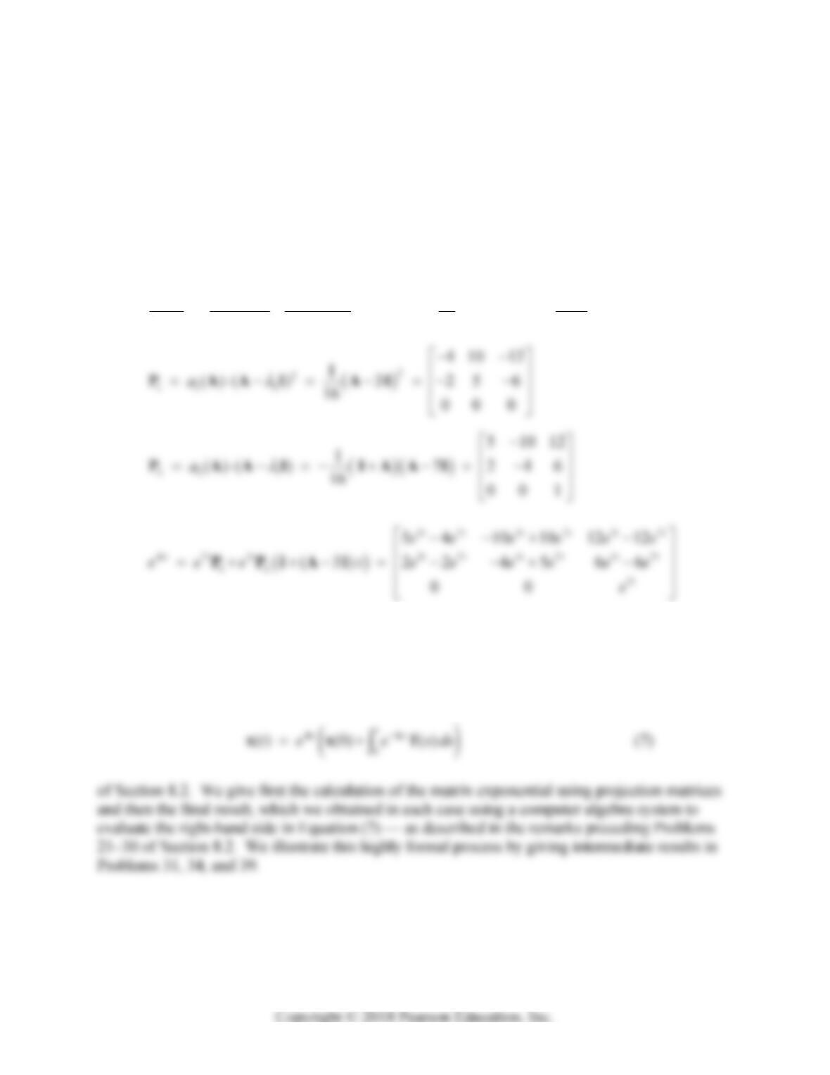
of multiplicity 2. We therefore use the method explained in Problem 19 above, and list here
the results of the principal steps in the calculation of the fundamental matrix .
t
eA
27. 2
12
200
797; () ( 9)( 2); 9, 2
002
p
A
500 Chapter 8: Matrix Exponential Methods
28. 2
12
25 12 0
18 5 0 ; ( ) ( 7)( 13) ; 7, 13
6613
p
A
12
2
1119 1 19
;(), ()
( ) 36( 9) 49( 3) 36 36
aa
p
713 713
713 713 713
12
7 13 7 13 13
23 22 0
(13) 3 3 3 2 0
tt tt
tt t tt tt
tt tt t
ee ee
eee t ee ee
ee ee e
APPIAI
29. 2
12
19 12 84
050; ()(9)(5); 9, 5
8433
p
A
Section 8.3: Spectral Decomposition Methods 501
59 59 5 9
95 5
12
59 59 59
7 6 3 3 21 21
(5) 0 0
22 67
tt tt t t
tt t t
tt tt tt
ee ee e e
eee t e
ee ee ee
APPIAI
30. 2
12
13 40 48
823 24; () ( 7)( 3); 7, 3
003
p
A
12
2
111 1 1
;(), ()
( ) 16( 7) 16( 3) 16 16
aa
p
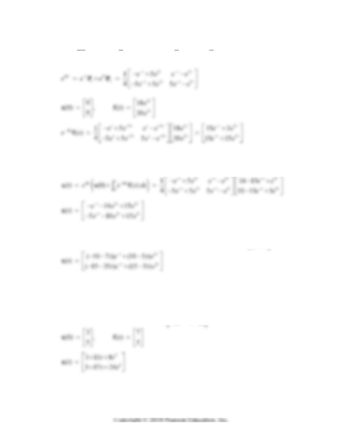
In Problems 31–40 we use the methods of this section to find the matrix exponentials that were
given in the statements of Problems 21–30 of Section 8.2. Once t
eA is known, the desired
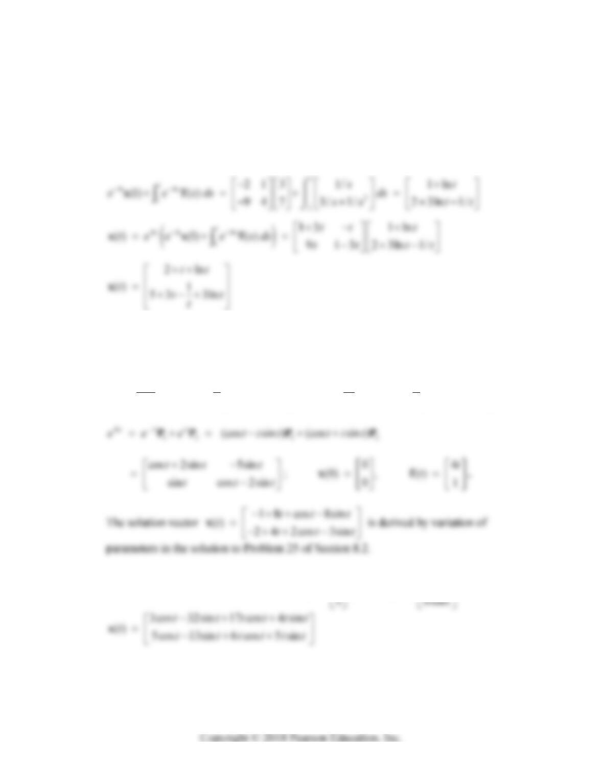
particular solution ( )tx is provided by the variation of parameters formula
31. 12
41
,1,3
52
A
502 Chapter 8: Matrix Exponential Methods
12
11 5 1
11 11
3,
55 5 1
44 44
PAI PAI
s
s
33
33
0
0
015 3 14 15
(0) ( ) 015 15 10 15 5
tss tt
ts
s
stt
ee ee
e s ds ds
ee ee
A
xf
32. With the same matrix exponential as in Problem 31, but with 3
28
() .
20
t
t
e
te
f
33. 12
31
,0, 0
93
A
013
(0) 913
tt tt
ee t t tt
AIA I IA (as in Problems 21-26)
Section 8.3: Spectral Decomposition Methods 503
34. With t
eA as in Problem 33, but with 2
30
(1) and ( ) .
71/
tt
xf Because
01,t we use the general variation of parameters formula in Eq. (25) of Section 8.2.
22
13 0 1/
() 9131/ 3/1/
sss s
es sss ss
Af
35. 12
25
,,
12 ii
A
12
12 5 12 5
11 11
,
12 12
22 22
ii ii
ii
ii ii
ii
PAI PAI
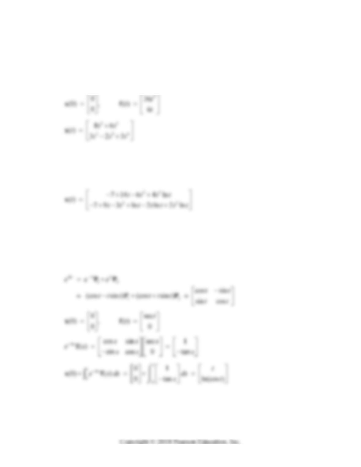
36. With t
eA as in Problem 35, but with 34cos
(0) and ( ) .
t
tt
x f
504 Chapter 8: Matrix Exponential Methods
37. 12
31
,0, 0
93
A
012 4
(0) 12
tt tt
ee t t tt
AIA I IA (as in Problems 21–26)
38. With t
eA as in Problem 37, but with 14ln
(1) and ( ) .
11/
t
tt
xf The details of
the variation of parameters process are similar to those shown in Problem 34 above.
39. 12
01
,,
10 ii
A
12
11
11 11
,
11
22 22
ii
ii
ii
ii
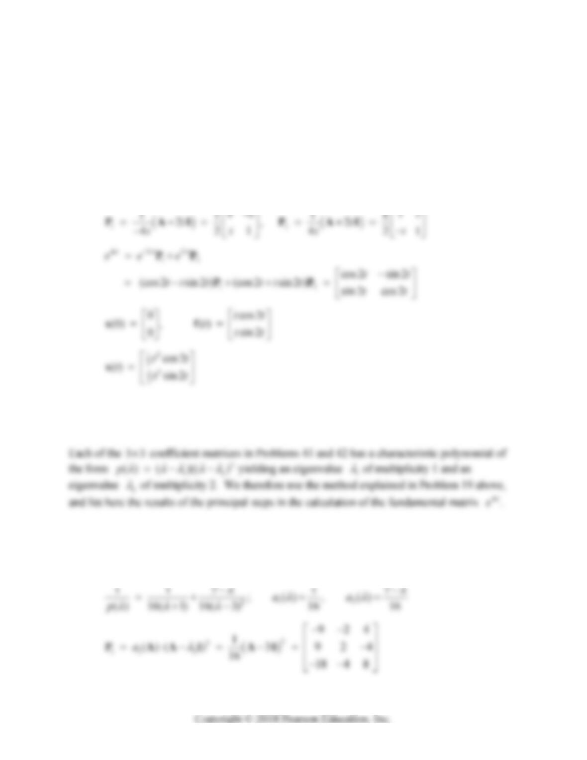
PAI PAI
Section 8.3: Spectral Decomposition Methods 505
0
cos sin
() (0) ( ) sin cos ln(cos )
t
ts ttt
te esds tt t
AA
xx f
cos ln(cos )sin
() sin ln(cos ) cos
tt t t
ttt t t
x
40. 12
02
,2,2
20 ii
A
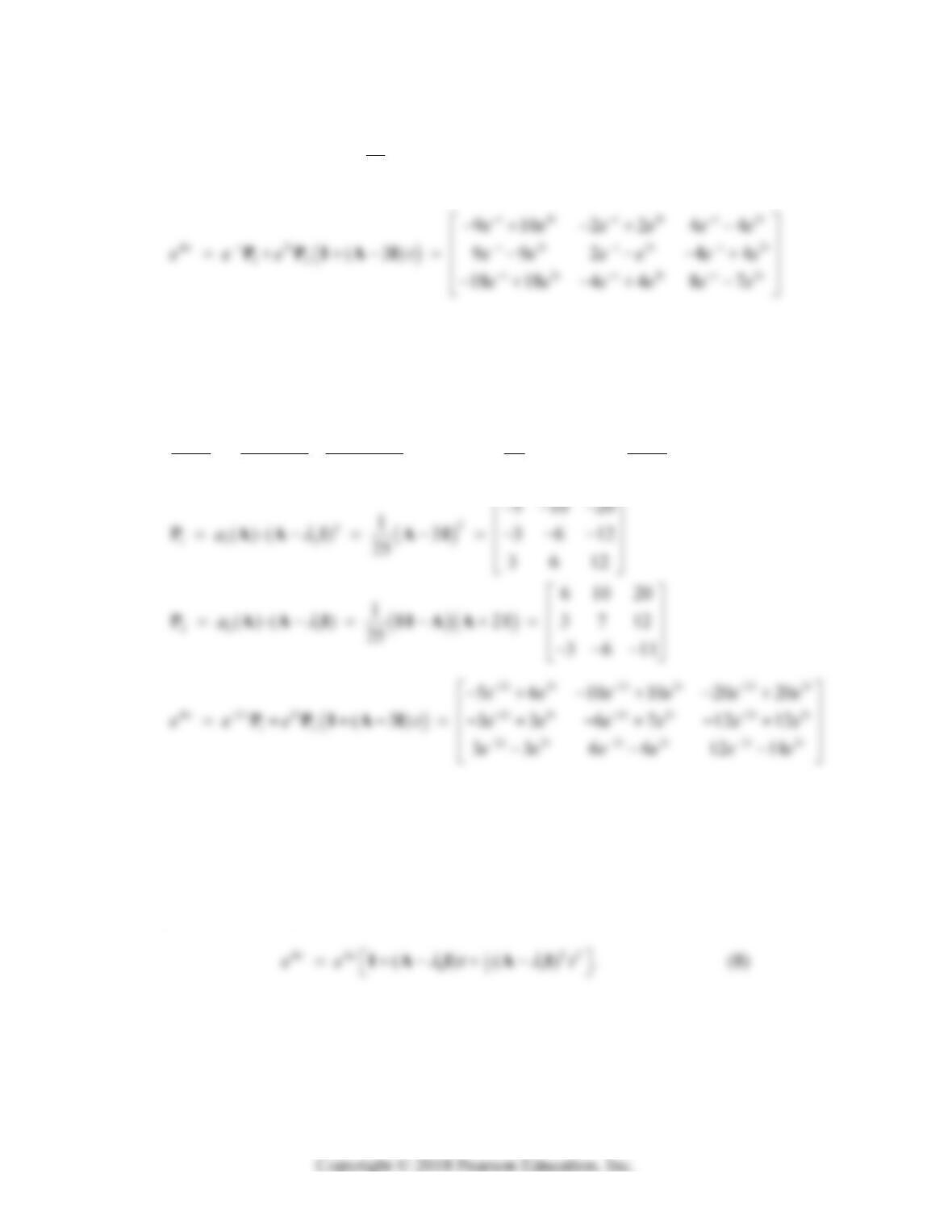
In Problems 41-46 we apply the methods of this section to compute the exponential matrices of
the coefficient matrices in Problems 23-26, 29, and 31 of Section 7.6.
41. 2
13
39 8 16
36 5 16 ; ( ) ( 1)( 3) , 1, 3
72 16 29
p
A
506 Chapter 8: Matrix Exponential Methods
22 1
10 2 4
1
()( ) 7 9 1 4
16 18 4 7
a
PAAI IAAI
42. 2
13
28 50 100
15 33 60 ; ( ) ( 2)( 3) , 2, 3
15 30 57
p
A
12
2
118 1 7
;(), ()
( ) 25( 1) 25( 3) 25 25
aa
p
In each of Problems 43 and 44, the given 33coefficient matrix A has characteristic
polynomial of the form 3
1
() ( )p
and thus a single eigenvalue 1
of multiplicity 3.
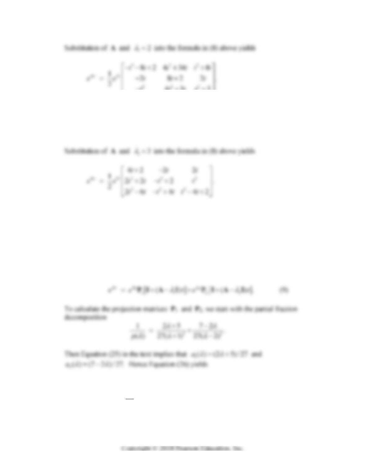
Consequently, Equations (25) and (26) in Section 8.3 of the text imply that 11
() () 1ab
and
hence that the associated projection matrix 1.PI Therefore Equation (35) in the text reduces
(with q = 1 and m1 = 3) to
43. 2
1
217 4
161; () ( 2), 2
012
p
A
Section 8.3: Spectral Decomposition Methods 507
tttt
44. 2
1
511
130; ()(3), 3
321
p
A
45. 22
12
11 1 2
74611
;()(1)(2), 1, 2
5113
6226
p
A
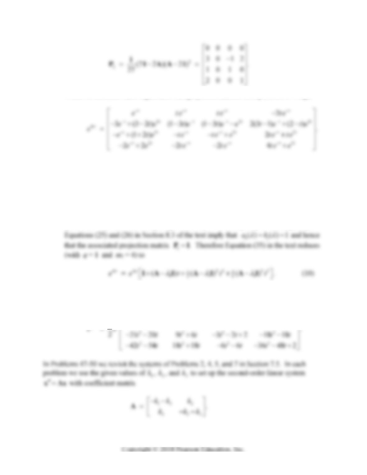
Since A has two eigenvalues 12
1and 2
each of multiplicity 2, Equation (35)
in the text reduces (with q = m1 = m2 = 2) to
2
1
1000
311 2
1(2 5 )( ) 100 0
27
200 0
PAIAI
and
508 Chapter 8: Matrix Exponential Methods
When we substitute these eigenvalues and projection matrices in Eq. (9) above we get
46. 4
1
35 12 4 30
22 8 3 19 ;()(1), 1
10 3 0 9
27 9 3 23
p
A
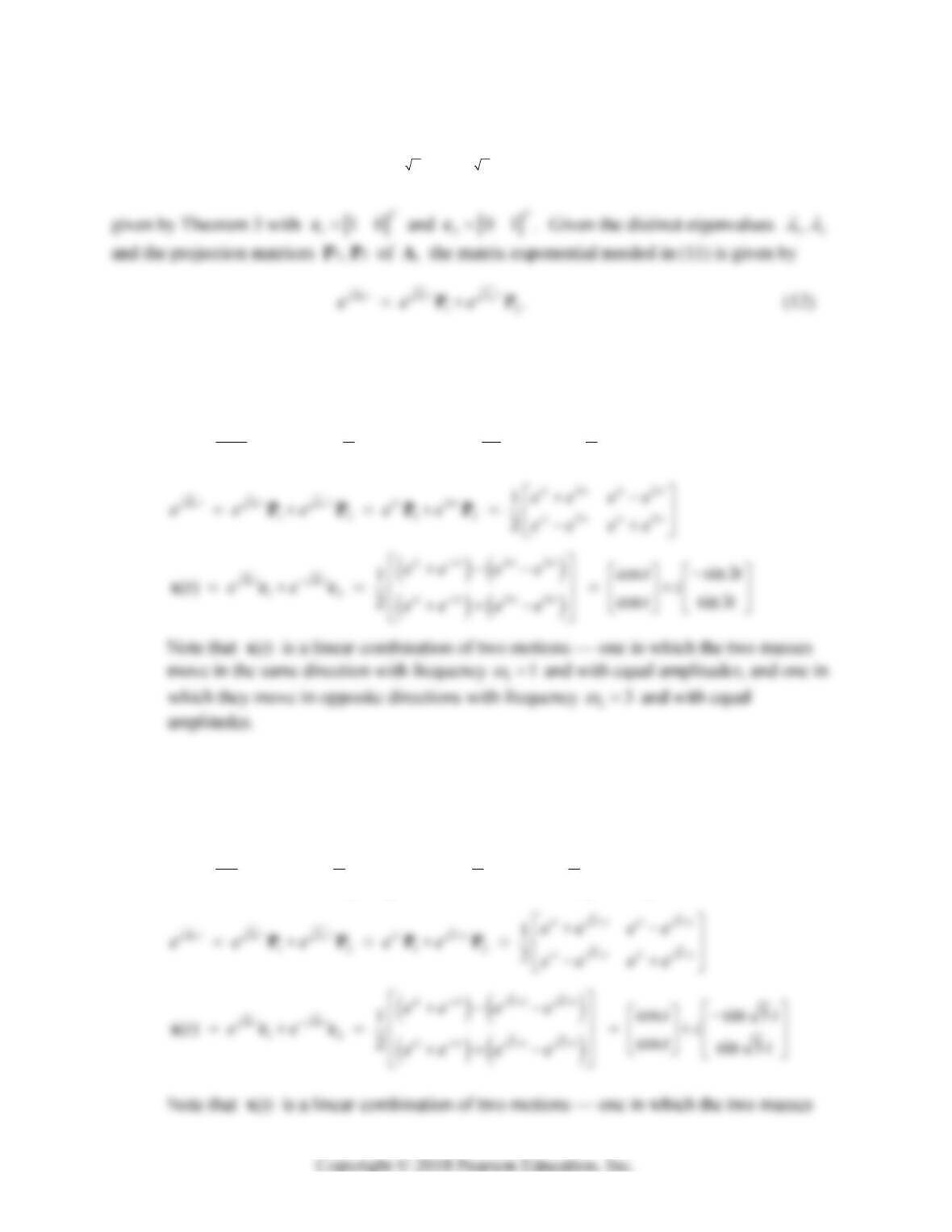
Thus the given 4 4coefficient matrix A has characteristic polynomial of the form
4
1
() ( )p
and thus a single eigenvalue 11
of multiplicity 4. Consequently,
When we substitute A and 11
in this formula we get
2222
22 2 2
48 68 2 18 24 6 8 36 60
744 3182 6 638
1.
tt
tt tt tt tt
tt tt tt tt
A
Section 8.3: Spectral Decomposition Methods 509
We then calculate the particular solution
12
() tt
te e
AA
xcc (11)
47. 2
12
54
;() 109, 1, 9
45 p
A
12
11 1 1
11 11
9,
11 1 1
10 2 10 2
PAI PAI
48. 2
12
32
;() 65, 1, 5
23 p
A
12
11 1 1
11 11
5,
11 1 1
62 62
PAI PAI
510 Chapter 8: Matrix Exponential Methods
49. 2
12
31
;() 68, 2, 4
13 p
A
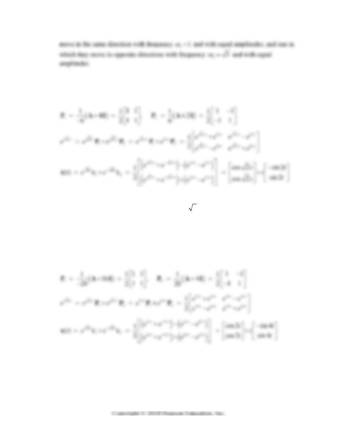
Note that x(t) is a linear combination of two motions — one in which the two masses
move in the same direction with frequency 12
and with equal amplitudes, and one
in which they move in opposite directions with frequency 22
and with equal
amplitudes.
50. 2
12
10 6 ; ( ) 20 64, 4, 16
610 p
A
Note that x(t) is a linear combination of two motions — one in which the two masses
move in the same direction with frequency 12
and with equal amplitudes, and one in
which they move in opposite directions with frequency 24
and with equal
amplitudes.
511
CHAPTER 9
NONLINEAR SYSTEMS AND PHENOMENA
SECTION 9.1
STABILITY AND THE PHASE PLANE
1. The only solution of the homogeneous system 20xy, 3 0xy is the origin
0, 0 .
2. The only solution of the system 0xy
, 340xy
is the point
1,1 . The only
figure among Figs. 9.1.12 through 9.1.19 showing a single critical point at
1,1 is Fig.
3. The only solution of the system 230xy
, 20xy is the point
1,1. The
only figure among Figs. 9.1.12 through 9.1.19 showing a single critical point at
1,1 is
4. The only solution of the system 2240xy
, 430xy
is the point
1, 1. The
only figure among Figs. 9.1.12 through 9.1.19 showing a single critical point at
1, 1 is
5. The first equation 2
10y
gives 1
y
or 1y at a critical point. Then the second
equation 2 0xy gives 2x or 2x, respectively. The only figure among Figs.
512 Chapter 9: Nonlinear Systems and Phenomena
6. The second equation 2
40x gives 2x or 2x at a critical point. Then the first
equation 2 4 15 0xy gives 2
5
y or 2
3
x, respectively. The only figure among
7. The first equation 3
40xx
gives 2x , 0x, or 2x at a critical point. Then the
second equation 20xy gives 1y , 0y, or 1y, respectively. The only figure
8. The second equation 20yx gives 2
y
x
at a critical point. Substitution of this in
the first equation 20xyx xy then gives 30xx, so 1x , 0x, or 1x.
In each of Problems 9-12 we need only set 0xx
and solve the resulting equation for x.
9. The equation
32
440xx x x has the three solutions 0, 2x. This gives the
three equilibrium solutions
0xt ,
2xt , and
2xt of the given 2nd-order dif-
Section 9.1: Stability and the Phase Plane 513
5
Problem 9
5
Problem 10
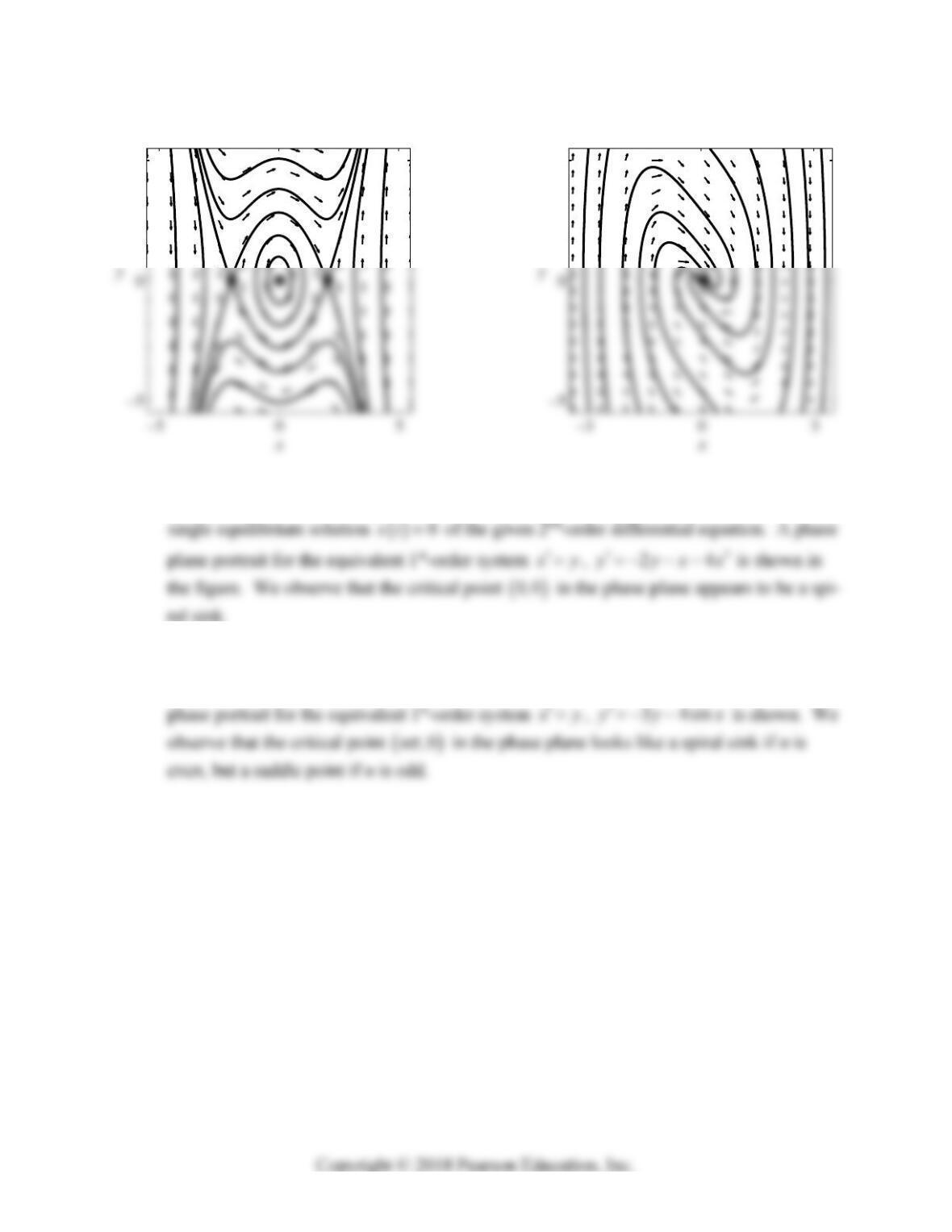
10. The equation
32
4140xxx x has the single real solution 0x. This gives the
11. The equation 4sin 0x is satisfied by
x
n
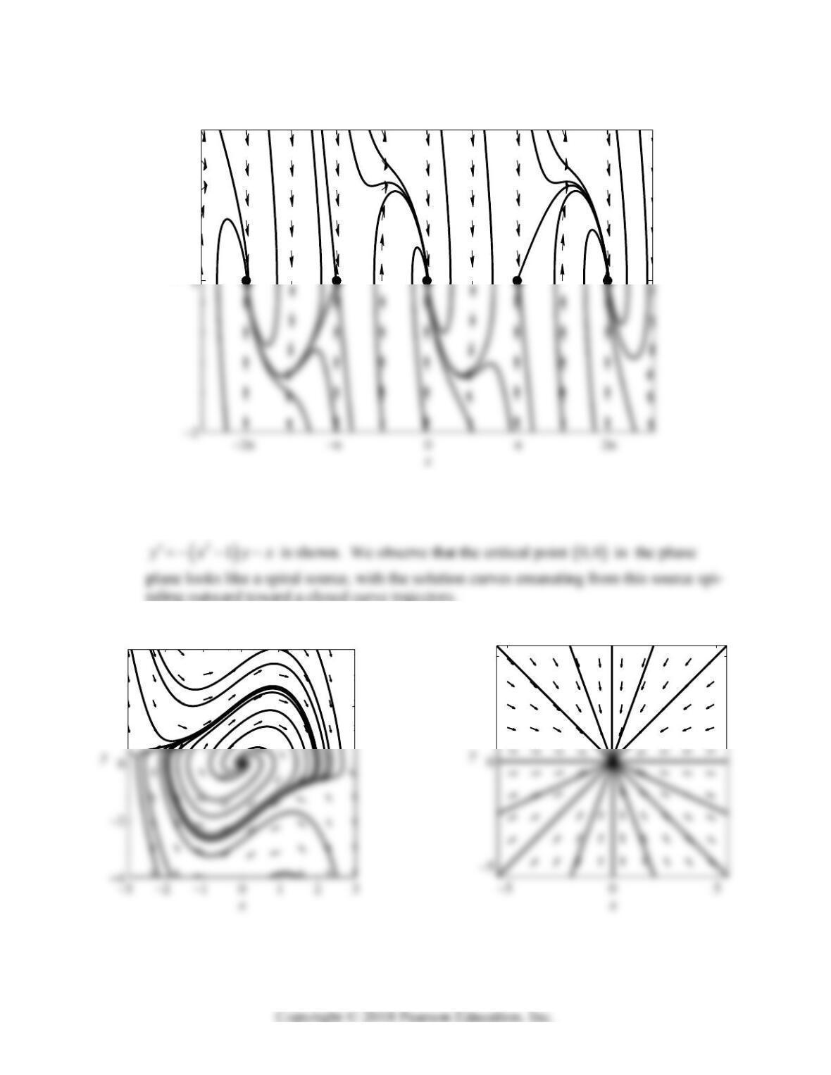
for any integer n. Thus the given 2nd–
order equation has infinitely many equilibrium solutions:
x
tn
for any integer n. A
514 Chapter 9: Nonlinear Systems and Phenomena
y
Problem 11
12. We immediately get the single solution 0x and thus the single equilibrium solution
0xt . A phase plane portrait for the equivalent 1st-order system
x
y
,
2
4
Problem 12
5
Problem 13