Section 5.5: Nonhomogeneous Equations and Undetermined Coefficients 315
37. 12 3
x
x
c
y
cce cxe ;
2
tr
x
yxAxBCxe
x
y
26
38.
12
cos sin
x
c
yec xc x
; tr cos3 sin 3
y
AxBx
y
y
85 85 85 85
39. 12 3
x
c
yccxce
;
2
tr
x
y
xABxxCe
23
x
y
x
40. 123 4 tr
cos sin ;
xx
c
yce cec xc xy A
g1 2 3 4
cos sin 5
xx
yce cec xc x
316 Chapter 5: Higher-Order Linear Differential Equations
41. The trial solution 2345
tr
y
ABxCxDxExFx leads to the equations
22624 0
2 2 6 24 120 0
AB C D E
BC D E F
42. The characteristic equation 432 20rrrr
has roots 1,2r , and i, so the
complementary function is 2
c1 2 3 4
cos sin
xx
y
ce ce c x c x
. We find that the coeffi-
cients satisfy the equations
43. (a) Applying Euler’s formula gives
332 23
cos3 sin 3 cos sin cos 3 cos sin 3cos sin sin
x
ix xix xi xx xxix .
When we equate real parts we get the equation
x
x
y
y
Section 5.5: Nonhomogeneous Equations and Undetermined Coefficients 317
The resulting general solution is
12
11
cos 2 sin 2 cos cos3
420
y
xc xc x x x .
44. We use the identity 11
22
sin sin 3 cos 2 cos 4
x
xxx, and hence substitute the trial solu-
tion cos2 sin 2 cos4 sin 4
p
y A xB xC xD x in the differential equation
y
y
45. We substitute
2
42
11 1
sin 1 cos2 1 2cos2 cos 2 3 4cos2 cos4
44 8
x
xxxxx
on the right-hand side of the differential equation, and then substitute the trial solution
46. By the formula for 3
cos
x
in Problem 43, the differential equation can be written as
31
cos cos3
44
y
yxxx x
.
The complementary solution is 12
cos sin
c
y
cxcx, so we substitute the trial solution
318 Chapter 5: Higher-Order Linear Differential Equations
2
1
13cos 3 sin
16
y
xxx x and
2
13sin3 4 cos3
128
y
xx x.
y
y
47. 2
1
x
y
e
, 2
x
y
e
, 3
x
We
, 3
1
4
3
x
ue , 2
22
x
ue, 2
3
x
p
y
e
x
x
x
50. The complementary function is 11 2
cosh 2 sinh 2
y
cxcx, so the Wronskian is
22
2cosh 2 2sinh 2 2Wxx
, so when we solve Equations (31) simultaneously for 1
u
2
u, integrate each, and substitute in 11 2 2p
yyuyu, the result is
11
cosh 2 sinh 2 sinh 2 sinh 2 cosh 2 sinh 2
22
p
y
xxxdxx xxdx
.
y
51. 1cos 2
y
x, 2sin 2
y
x, 2W. Liberal use of trigonometric sum and product identities
yields
1
1cos5 5cos
20
uxx
and
2
1sin 5 5sin
20
uxx
.
Section 5.5: Nonhomogeneous Equations and Undetermined Coefficients 319
52. 1cos3
y
x, 2sin 3
y
x, 3W;
1
16sin6
36
uxx ,
2
11cos6
36
ux ;
11
6sin6cos3 1cos6sin3
36 36
p
yxxx xx
53. 1cos3
y
x, 2sin 3
y
x, 3W; 1
2tan 3
3
ux
, so 1
2ln cos3
9
ux; 2
2
3
u, so
2
2
3
ux. Thus
y
54. 1cos
y
x, 2sin
y
x, 1W; 1cscux
, so 1ln csc cotuxx ; 2
2cos cscuxx
,
so 2cscux . Thus
ln csc cot cos csc sin 1 cos ln csc cot
p
yxxxxx xxx .
y
y
320 Chapter 5: Higher-Order Linear Differential Equations
so
2
1
12cos2 cos 2
16
uxx;
2 2
2
111cos21 1
sin cos 2 cos 2 cos 2 cos 2 2 cos 2 1 cos 4
2224 8
x
uxx x xx x x
,
x
because the single-underlined terms sum to 2. The double-underlined terms reduce to
y
y
33
32
11
cos 2 sin 4 sin 2 cos 2 2sin 2 cos2 sin 2
22
cos 2 sin 2 cos2
x
xx x x x x
xxx
56. 2
1
x
y
e
, 2
2
x
y
e, 4W;
3
1
131
36
x
uxe ;
2
11
4
x
uxe
;
132
9
x
p
yxe .
y
Section 5.5: Nonhomogeneous Equations and Undetermined Coefficients 321
4165
11 2 2 963
p
y
yu yu x x x x x
.
58. Here it is important to remember that in order to apply the method of variation of parame-
ters, the differential equation must be written in standard form with leading coefficient 1.
We therefore rewrite the given equation with complementary function 23
12c
ycxcx as
f
59. 2
1
y
x, 2
2ln
y
xx, 3
Wx,
2
f
xx; 1lnuxx
, 2
ux
; 4
1
4
p
y
x.
f
61.
1cos ln
y
x,
2sin ln
y
x, 1
W
x
,
2
ln
x
fx
x
; from
1
ln sin ln
x
x
ux
and
2
ln cos ln
x
x
ux
integration by parts yields
x
x
1
ln sin ln sin ln ln
xx x
udxxdx
xx
322 Chapter 5: Higher-Order Linear Differential Equations
62. 1
y
x, 2
21
y
x , 21Wx,
1fx. From
2
12
1
1
x
u
x
, long division and the
method of partial fractions yield
x
x
63. This is simply a matter of solving the equations in (31) for the derivatives
y
y
64. Here we have
1cos
y
xx,
2sin
y
xx,
1Wx, and
2sin
f
xx, so (33) gives
x
y
cos sin 2sin sin cos 2sin
p
y
xxxxdxxxxdx
SECTION 5.6
FORCED OSCILLATIONS AND RESONANCE
1. Trial of cos2
x
At yields the particular solution 2cos2
p
x
t. (Can you see that be-
cause the differential equation contains no first-derivative term, there is no need to in-
clude a sin 2t term in the trial solution?) Hence the general solution is
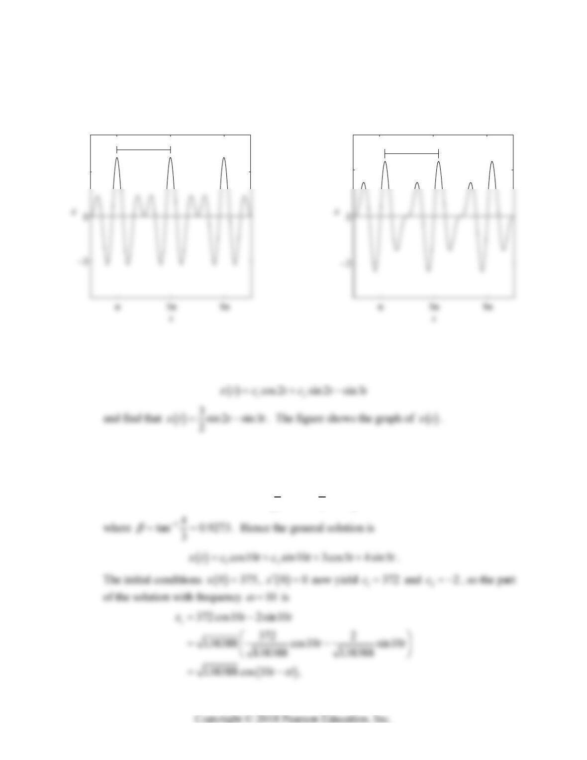
Section 5.6: Forced Oscillations and Resonance 323
The initial conditions imply that 12c and 20c, so
2cos2 2cos3
x
ttt. The
figure shows the graph of
x
t.
Problem 1
Problem 2
2. Trial of sin 3
x
At yields the particular solution sin 3
p
x
t . Then we impose the ini-
tial conditions
000xx
on the general solution
x
x
x
3. First we apply the method of undetermined coefficients with trial solution
cos5 sin5
x
AtBt to find the particular solution
34
3cos 5 4sin 5 5 cos 5 sin 5 5cos 5
55
p
xtt tt t
,
x
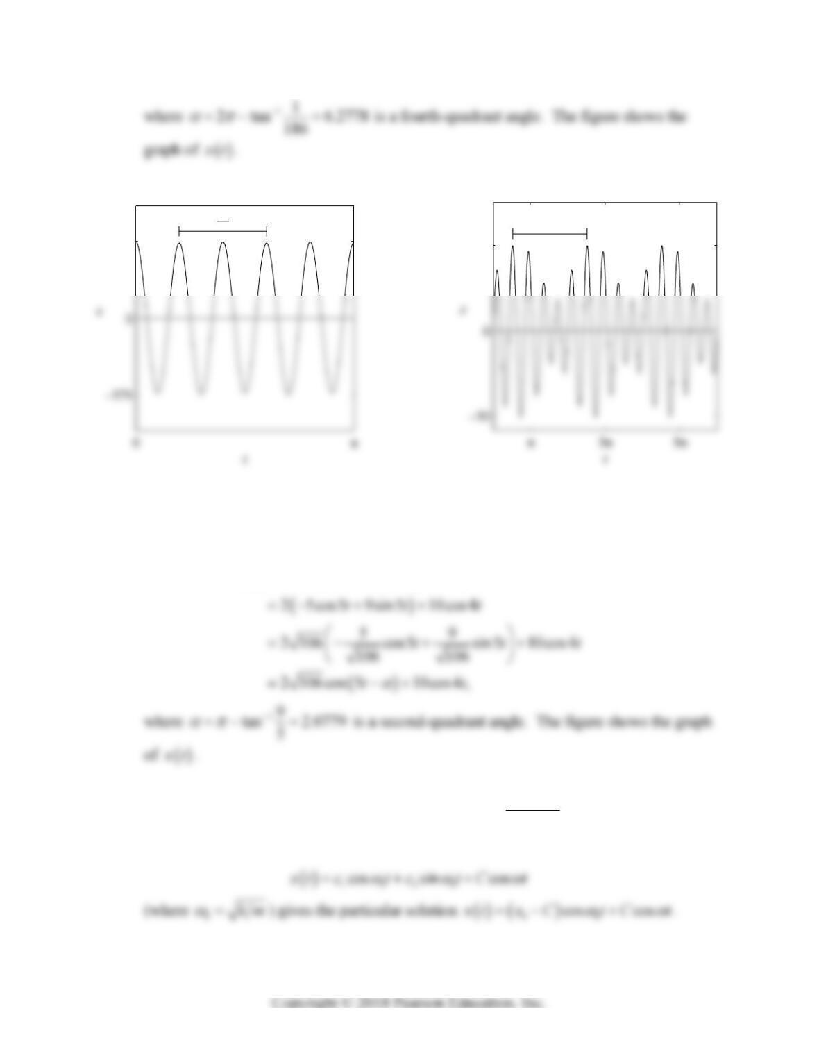
324 Chapter 5: Higher-Order Linear Differential Equations
x
2π
5
Problem 3
2π
Problem 4
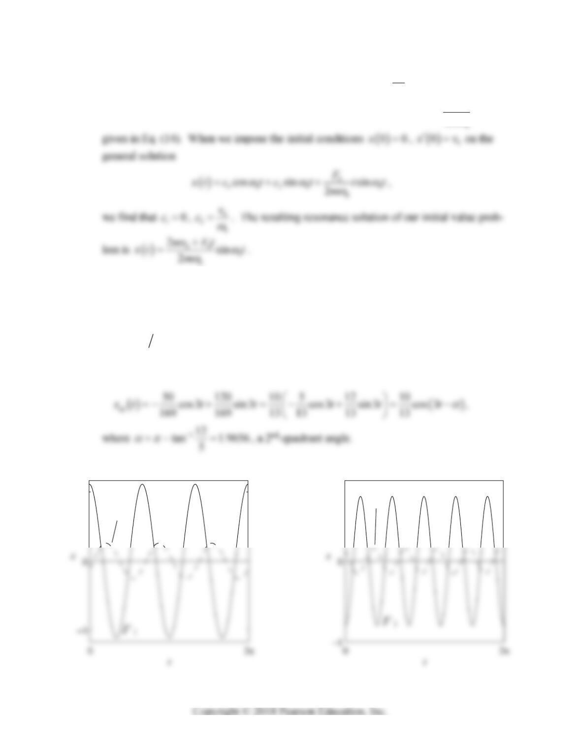
4. Noting that there is no first-derivative term, we try cos4
x
At and find the particular
solution 10cos4
p
x
t. Then imposition of the initial conditions on the general solution
12
cos5 sin5 10cos4
x
tc tc t t yields
x
10 cos5 18sin 5 10 cos 4
xt t t t
5. Substitution of the trial solution cos
x
Ct
gives 0
2
F
Ckm
. Then imposition of the
initial conditions
0
0
x
x,
00x on the general solution
x
x
Section 5.6: Forced Oscillations and Resonance 325
6. First, let’s write the differential equation in the form 20
00
cos
F
x
xt
m
, which is the
same as Eq. (13) in the text, and therefore has the particular solution 0
0
x
x
x
sin
2
p
F
x
tt
m
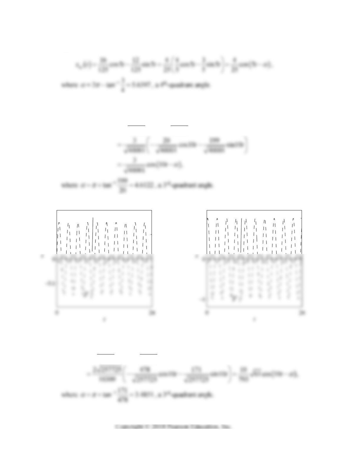
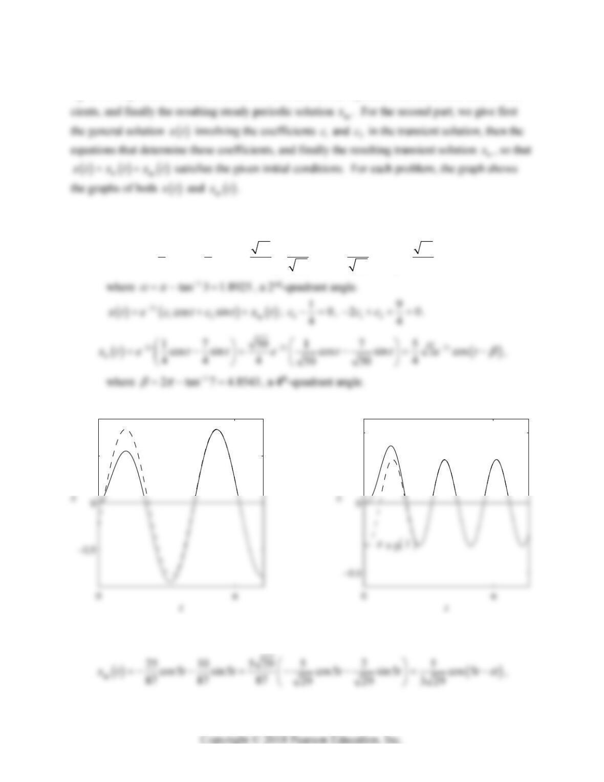
In Problems 7–10 we give first the trial solution p
x
involving undetermined coefficients A and
B, then the equations that determine these coefficients, and finally the resulting steady periodic
solution sp
x
. In each case the figure shows the graphs of
sp
x
t and the adjusted forcing func-
tion
1()Ft Ft m
.
7. cos3sin3
p
x
AtBt; 512 10AB , 12 5 0AB.
xsp
Problem 7
xsp
Problem 8
326 Chapter 5: Higher-Order Linear Differential Equations
8. cos5sin5
p
x
AtBt; 20 15 4AB , 15 20 0AB.
9. cos10 10sin10
p
x
At t; 199 20 0AB, 20 199 3AB.
sp
60 597
cos10 sin10
40001 40001
xt t t
xsp
Problem 9
xsp
Problem 10
10. pcos10 10sin5
x
At t; 97 30 8AB , 30 97 6AB.
sp
956 342
cos10 sin10
10309 10309
xt t t
Section 5.6: Forced Oscillations and Resonance 327
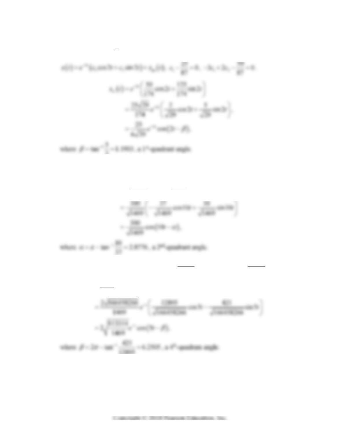
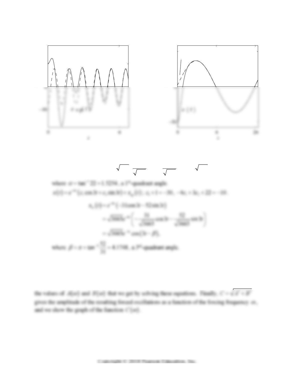
Each solution in Problems 11–14 has two parts. For the first part, we give first the trial solution
p
x
involving undetermined coefficients A and B, then the equations that determine these coeffi-
x
x
11. pcos3 sin 3
x
AtBt; 41210AB , 12 4 0AB
.
sp
1 3 10 1 3 10
cos3 sin 3 cos3 sin 3 cos 3
44 4 4
10 10
xt t t t t t
,
xsp
(t)
x(t)
Problem 11
x(t)
Problem 12
12. cos5sin5
p
x
AtBt; 12 30 0AB
, 30 12 10AB
.
328 Chapter 5: Higher-Order Linear Differential Equations
where 12
tan 3.5221
5
, a 3rd-quadrant angle.
x
2
13. cos10 sin10
p
x
AtBt
; 74 20 600AB, 20 74 0AB.
sp
11100 3000
cos10 sin10
1469 1469
xt t t
12 sp
cos5 sin 5
t
x
tec tc txt
; 1
11100 10
1469
c, 12
30000
51469
cc .
tr 25790cos5 842sin 5
1469
t
e
xt t t
12895
Section 5.6: Forced Oscillations and Resonance 329
x
x(t)
Problem 13
x
xsp
(t)
Problem 14
14. cos sin
p
x
AtBt
; 24 8 200AB , 824 520AB .
sp
122
cos 22sin 485 cos sin 485 cos
485 485
xt t t t t t
,
x
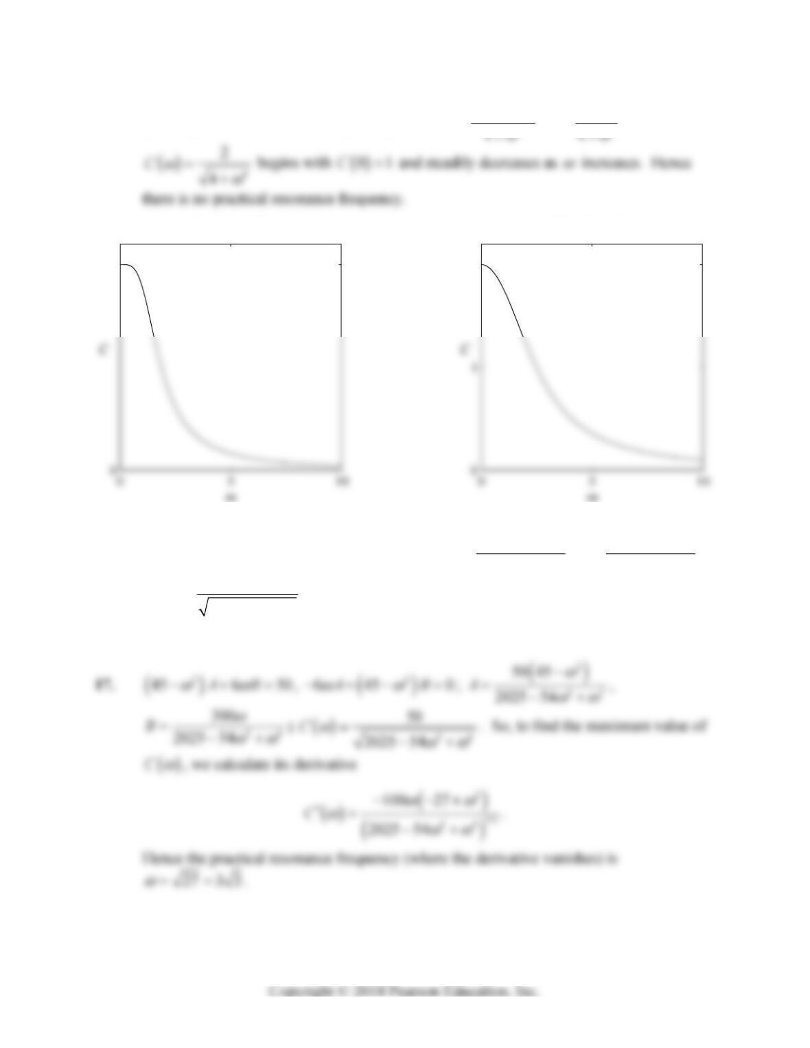
In Problems 15-18 we substitute
cos sin
x
tA tB t
into the differential equation
0cosmx cx kx F t
with the given numerical values of m, c, k, and 0
F. We give first the
equations in A and B that result upon collection of coefficients of cos t
and sin t
, followed by
330 Chapter 5: Higher-Order Linear Differential Equations
15.
2
222AB
,
2
22 0AB
;
2
4
22
A
, 4
4
B
;
1
Problem 15
2
Problem 16
16.
2
5410AB
,
2
45 0AB
;
2
24
10 5
25 6
A
, 24
40
25 6
B
;
24
10
25 6
C
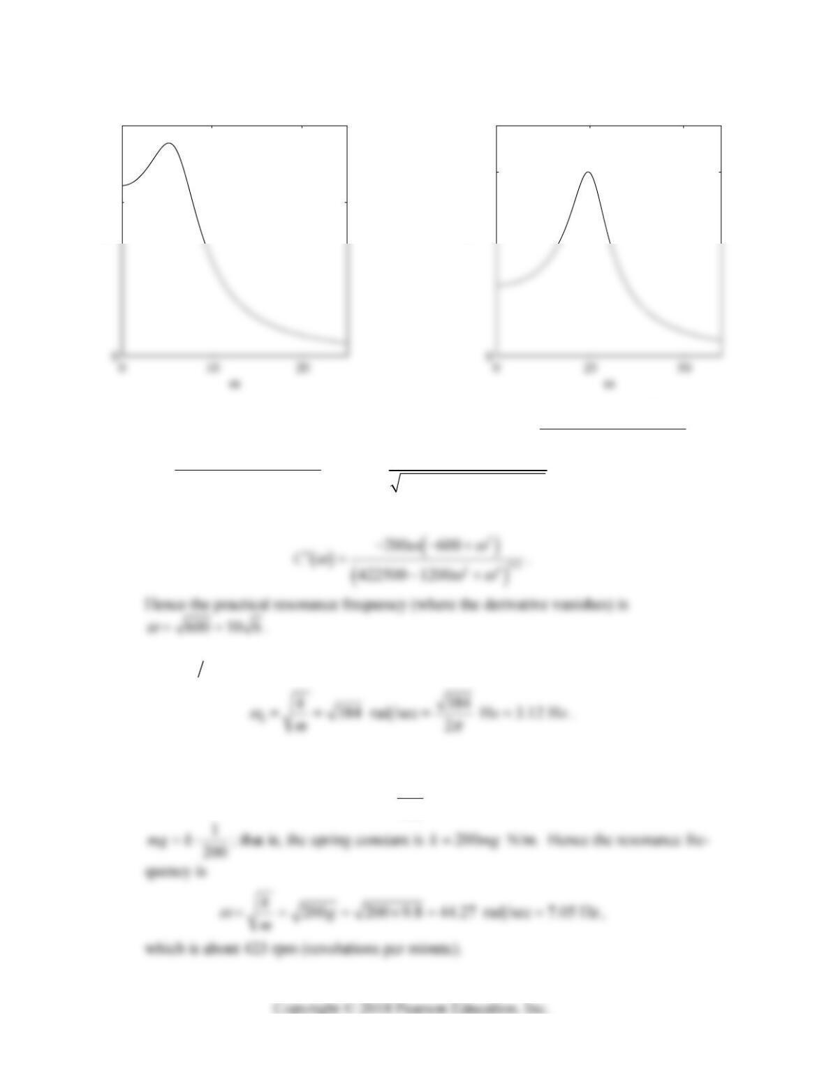
begins with
02C and steadily decreases as
increases.
Hence there is no practical resonance frequency.
Section 5.6: Forced Oscillations and Resonance 331
1
C
Problem 17
0.4
C
Problem 18
18.
2
650 10 100AB
,
2
10 650 0AB
;
2
24
100 650
422500 1200
A
,
24
1000
422500 1200
B
;
24
100
422500 1200
C
. So, to find the maximum
value of
C
, we calculate its derivative
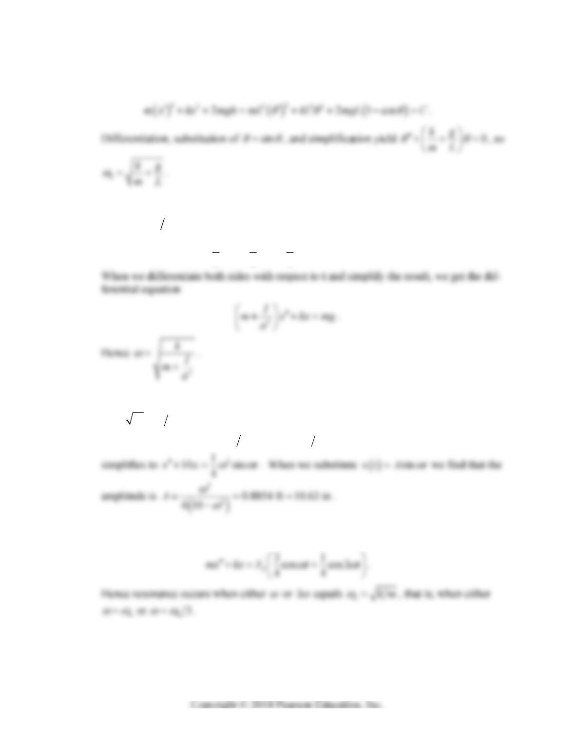
19. 100 32m slugs and 1200k lb/ft, so the critical frequency is
20. Let the machine have mass m. Then the force 9.8 mFmg (the machine’s weight)
causes a displacement of 1
0.5 cm m
200
x , so Hooke’s law Fkx gives
332 Chapter 5: Higher-Order Linear Differential Equations
21. If
is the angular displacement from the vertical, then the (essentially horizontal) dis-
placement of the mass is
x
L
, so twice its total energy (KE + PE) is
22. Let x denote the displacement of the mass from its equilibrium position, vx
its veloci-
ty, and va
the angular velocity of the pulley. Then conservation of energy yields
222
111
222
mv I kx mgx C
.
23. (a) In units of ft-lb-sec we have 1000m and 10000k, so
010 rad sec 0.50 Hz
.
(b) We are given that 2 2.25 2.79 rad sec
, and the equation
mx kx F t
24. By the identity of Problem 43 in Section 5.5, the differential equation is
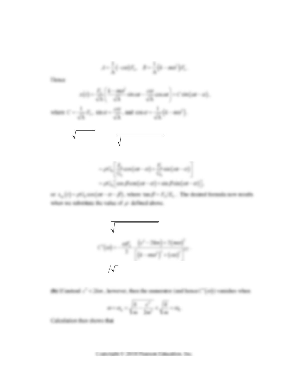
25. Substitution of the trial solution cos sin
x
AtBt
in the differential equation fol-
lowed by collection of coefficients as usual yields the equations
Section 5.6: Forced Oscillations and Resonance 333
22
0
0,km AcB cAkm BF
with coefficient determinant
22
2
km c
and solution
26. Let 22
000
GEF
and
2
2
1
km c
. Then
sp 0 0
cos( ) sin( )
xt E t F t
27. The derivative of
0
22
2
F
C
km c
is given by
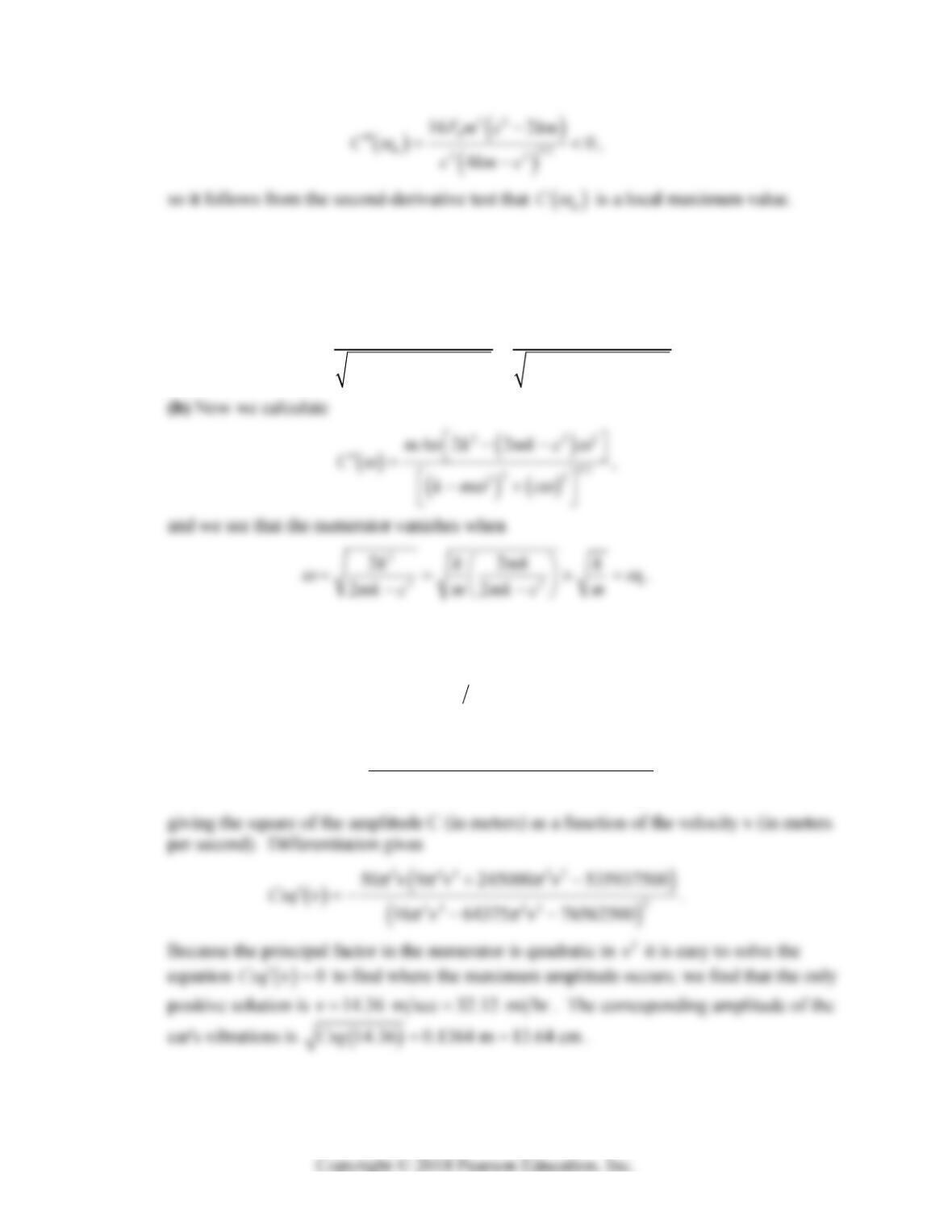
(a) Therefore, if
2
2
cr 22cc km, it is clear from the numerator that
0C
for
all
, so that
C
steadily decreases as
increases.
334 Chapter 5: Higher-Order Linear Differential Equations
28. (a) The given differential equation corresponds to Equation (17) with 2
0
FmA
. It
therefore follows from Equation (21) that the amplitude of the steady periodic vibrations
at frequency
is
2
0
22
22
22
FmA
C
km c km c
.
29. We need only substitute 0
Eac
and 0
Fak in the result of Problem 26.
30. When we substitute the values 2vL
, 800m, 4
710k , 3000c, 10L, and
0.05a in the formula of Problem 29, simplify, and square, we get the function
22
2
44 22
25 9 122500
16 16 64375 76562500
v
Csq v
vv