INSTRUCTOR’S
SOLUTIONS MANUAL
DIFFERENTIAL EQUATIONS
& LINEAR ALGEBRA
FOURTH EDITION
C. Henry Edwards
The author and publisher of this book have used their best efforts in preparing this book. These efforts include the
development, research, and testing of the theories and programs to determine their effectiveness. The author and publisher
make no warranty of any kind, expressed or implied, with regard to these programs or the documentation contained in this
book. The author and publisher shall not be liable in any event for incidental or consequential damages in connection with,
or arising out of, the furnishing, performance, or use of these programs.
ISBN–13: 978-0-13–449825-6
ISBN–10: 0–13–449825-9
iii
CONTENTS
1 FIRST-ORDER DIFFERENTIAL EQUATIONS
1.1 Differential Equations and Mathematical Models 1
1.2 Integrals as General and Particular Solutions 8
2 MATHEMATICAL MODELS
AND NUMERICAL METHODS
2.1 Population Models 101
2.2 Equilibrium Solutions and Stability 117
3 LINEAR SYSTEMS AND MATRICES
3.1 Introduction to Linear Systems 173
3.2 Matrices and Gaussian Elimination 177
iv
4 VECTOR SPACES
4.1 The Vector Space
3
R 229
4.2 The Vector Space Rnand Subspaces 235
5 HIGHER-ORDER LINEAR
DIFFERENTIAL EQUATIONS
5.1 Introduction: Second-Order Linear Equations 275
5.2 General Solutions of Linear Equations 282
6 EIGENVALUES AND EIGENVECTORS
6.1 Introduction to Eigenvalues 335
7 LINEAR SYSTEMS OF
DIFFERENTIAL EQUATIONS
7.1 First-Order Systems and Applications 379
7.2 Matrices and Linear Systems 388
v
8 MATRIX EXPONENTIAL METHODS
8.1 Matrix Exponentials and Linear Systems 473
9 NONLINEAR SYSTEMS AND PHENOMENA
9.1 Stability and the Phase Plane 511
9.2 Linear and Almost Linear Systems 520
10 LAPLACE TRANSFORM METHODS
10.1 Laplace Transforms and Inverse Transforms 565
10.2 Transformation of Initial Value Problems 570
11 POWER SERIES METHODS
11.1 Introduction and Review of Power Series 609
APPENDIX A
Existence and Uniqueness of Solutions 649
vi
Copyright © 2018 Pearson Education, Inc.
PREFACE
This is a solutions manual to accompany the textbook DIFFERENTIAL EQUATIONS &
LINEAR ALGEBRA (4th edition, 2018) by C. Henry Edwards, David E. Penney, and David T.
Calvis. We include solutions to most of the problems in the text. The corresponding Student’s
Solutions Manual contains solutions to most of the odd-numbered solutions in the text.
1
CHAPTER 1
FIRST-ORDER DIFFERENTIAL EQUATIONS
SECTION 1.1
DIFFERENTIAL EQUATIONS AND MATHEMATICAL MODELS
The main purpose of Section 1.1 is simply to introduce the basic notation and terminology of dif-
ferential equations, and to show the student what is meant by a solution of a differential equation.
Also, the use of differential equations in the mathematical modeling of real-world phenomena is
outlined.
Problems 1-12 are routine verifications by direct substitution of the suggested solutions into the
given differential equations. We include here just some typical examples of such verifications.
y
y
y
y
y
y
x
x
x
x
5. If
x
x
y
ee
, then
x
x
y
ee
, so
2.
xx xx x
yy
ee ee e
Thus
2.
x
y
ye
6. If 2
1
x
ye
and 2
2
x
yxe
, then 2
12
x
ye
, 2
14
x
ye
, 22
22
x
x
ye xe
, and
22
244.
x
x
yexe
Hence
y
y
y
y
y
y
2 Chapter 1: First-Order Differential Equations
11. If 2
1
yy x
, then 3
2
y
x
and 4
6,
y
x
so
y
y
13. Substitution of rx
y
e into
32
yy
gives the equation 3 2
rx rx
re e, which simplifies
to 32.r Thus 2/3r.
y
y
16. Substitution of rx
y
e into 3340yyy
gives the equation
2
3340,
rx rx rx
re re e which simplifies to 2
3340rr
. The quadratic formula then
gives the solutions
3576r .
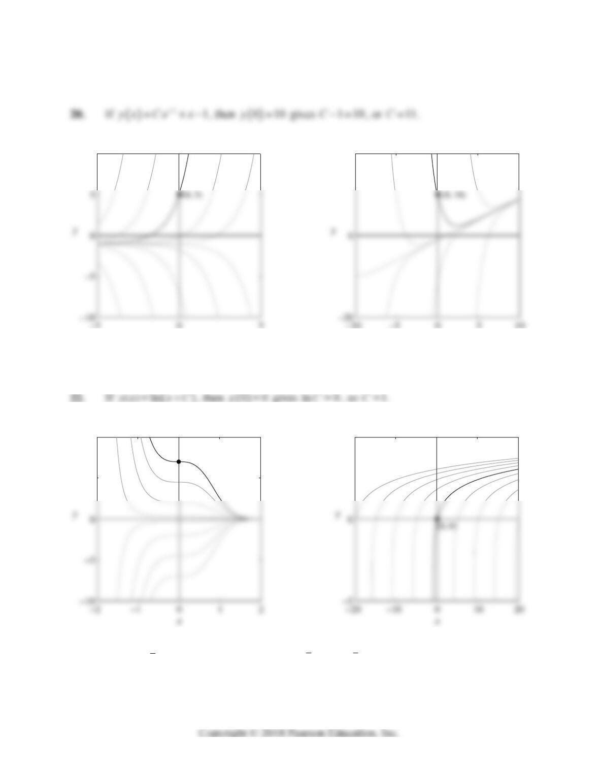
17. 2C 18. 3C
4
(0, 2)
Problem 17
5
(0, 3)
Problem 18
Section 1.1: Differential Equations and Mathematical Models 3
19. If
1
x
yx Ce
, then
05y gives 15C , so 6C.
21. 7C.
23. If 52
1
4
()yx x Cx
, then
21y gives 11
48
32 1C, or 56C .
24. 17C.
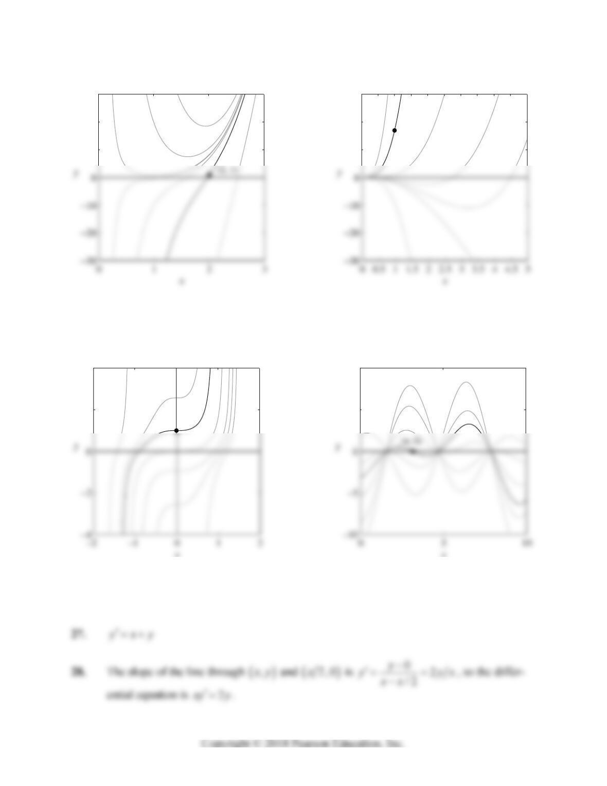
10
x
Problem 19
20
x
Problem 20
5
10
(0, 7)
Problem 21
5
Problem 22
4 Chapter 1: First-Order Differential Equations
25. If
3
tan
y
xC
, then
01y gives the equation tan 1C. Hence one value of C is
/4C
, as is this value plus any integral multiple of
.
26. Substitution of
x
and 0y into
cosyxC x yields
01C
, so
C
.
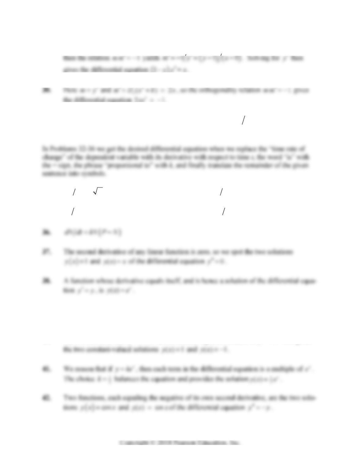
10
20
30
Problem 23
10
20
30
(1, 17)
Problem 24
2
4
x
(0, 1)
Problem 25
5
10
x
Problem 26
Section 1.1: Differential Equations and Mathematical Models 5
29. If m
y
is the slope of the tangent line and m is the slope of the normal line at (, ),
xy
y
31. The slope of the line through
,
x
y and (,)
y
x is
yxy yx
, so the differen-
tial equation is () .
xyy y
x
32. dP dt k P 33.
2
dv dt kv
34.
250dv dt k v
35.
dN dt k P N
y
y
39. We reason that if 2
y
kx, then each term in the differential equation is a multiple of 2
x
.
The choice 1k balances the equation and provides the solution 2
()
y
xx.
40. If y is a constant, then 0y, so the differential equation reduces to 21y. This gives
y
6 Chapter 1: First-Order Differential Equations
43. (a) We need only substitute
() 1
x
tCkt
in both sides of the differential equation
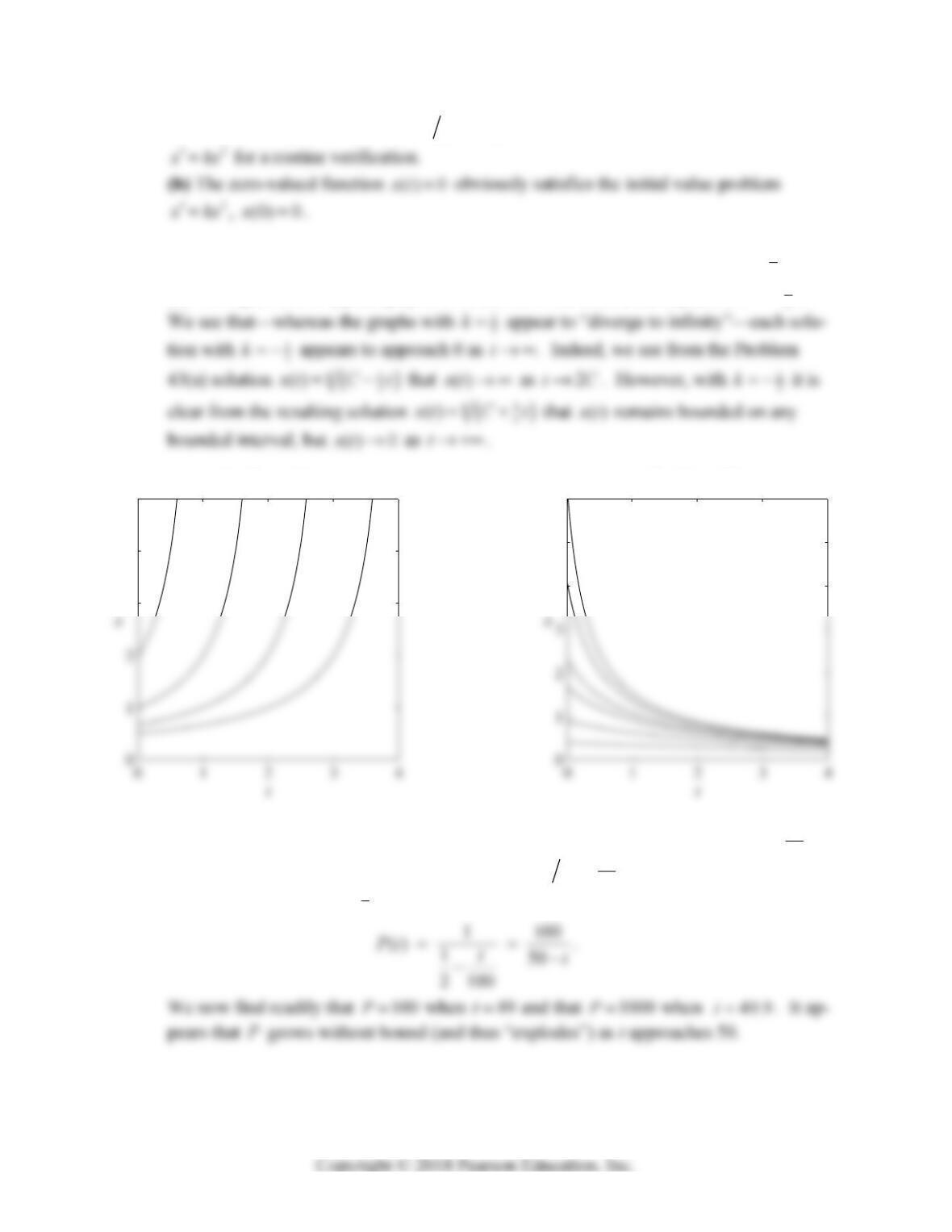
44. (a) The figure shows typical graphs of solutions of the differential equation 2
1
2
x
x
.
(b) The figure shows typical graphs of solutions of the differential equation 2
1
2.
x
x
x
x
45. Substitution of 1P and 10P into the differential equation 2
PkP
gives 1
100 ,k so
Problem 43(a) yields a solution of the form
1
100
() 1Pt C t. The initial condition
(0) 2P
now yields 1
2,C so we get the solution
3
4
5
Problem 44a
4
5
6
Problem 44b
Section 1.2: Integrals as General and Particular Solutions 7
46. Substitution of 1v and 5v into the differential equation 2
vkv
gives 1
25 ,k so
Problem 43(a) yields a solution of the form
() 1 25vt C t . The initial condition
47. (a)
(10) 10y
yields
10 1 10C
, so 101 10C.
(b) There is no such value of C, but the constant function () 0yx satisfies the conditions
48. (b) Obviously the functions 4
()ux x and 4
()vx x both satisfy the differential equa-
tion 4.
xy y
But their derivatives 3
() 4ux x
and 3
() 4vx x
match at 0x, where
both are zero. Hence the given piecewise-defined function
yx is differentiable, and
8 Chapter 1: First-Order Differential Equations
SECTION 1.2
INTEGRALS AS GENERAL AND PARTICULAR SOLUTIONS
This section introduces general solutions and particular solutions in the very simplest situation
— a differential equation of the form
yfx
— where only direct integration and evaluation
of the constant of integration are involved. Students should review carefully the elementary con-
cepts of velocity and acceleration, as well as the fps and mks unit systems.
1. Integration of
21
y
x
yields
2
() 2 1
y
xxdxxxC
. Then substitution of
0x, 3y gives 300CC , so
23yx x x
.
y
y
4. Integration of 2
y
x
yields
21
y
xxdx xC
. Then substitution of 1
x
,
5y gives 51C , so
16yx x .
y
7. Integration of 2
10
1
yx
yields
1
2
10 10 tan
1
yx dx x C
x
. Then substitution of
0x, 0y gives 0100C
, so
1
10 tanyx x
.
y
y
Section 1.2: Integrals as General and Particular Solutions 9
10. Integration of
x
y
xe
yields
11
xu u x
y
xxedxueduue xeC
,
using the substitution ux together with Formula #46 inside the back cover of the
textbook. Then substituting 0x,
1
y
gives 11,C so ( ) ( 1) 2.
x
yx x e
x
13. If
3at t, then
22
33
0
22
35vt tdt t v t
. Hence
23 3
311
0
22 2
55 5
x
ttdtttxtt
.
x
16. If
1
4
at t
, then
124 245
4
vt dt t C t
t
(taking 5C so
that
01v ). Hence
10 Chapter 1: First-Order Differential Equations
17. If
3
1at t
, then
32 2
111
222
11 1vt t dt t C t
(taking
18. If
50sin 5at t, then
50sin 5 10 cos5 10cos 5vt tdt t C t
(taking 0C so
that
010v ). Hence
10cos5 2sin 5 2sin 5 10xt tdt t C t
x
19. The graph of
vt shows that
5if 05
10 if 5 10
t
vt tt
, so that
1
2
1
2
2
5if 05
10 if 5 10
tC t
xt ttC t
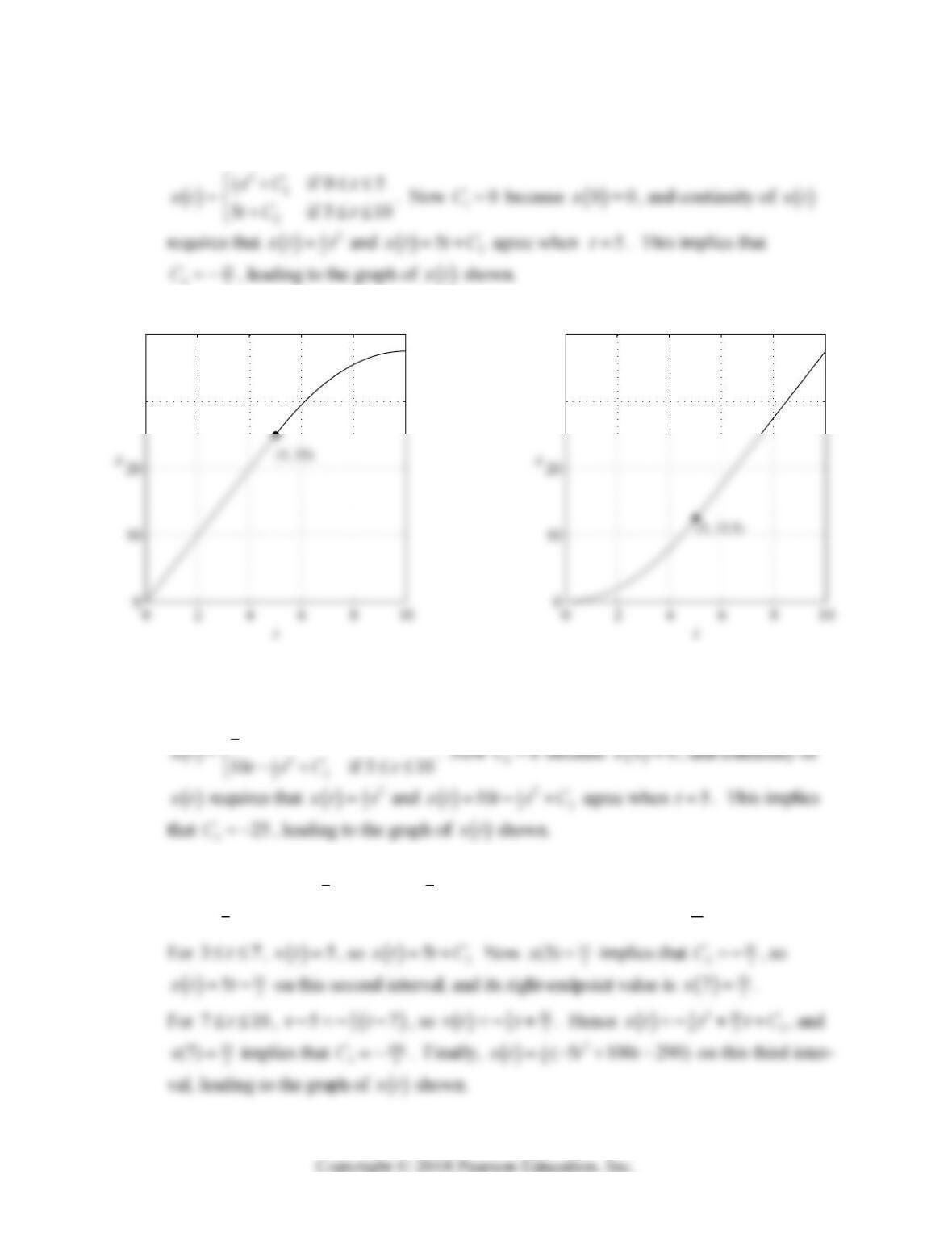
. Now 10C because
00x, and continuity of
x
t requires that
5
x
tt and
2
1
2
2
10
x
tttC
agree when 5t. This implies
that 25
22
C , leading to the graph of
x
t shown.
Alternate solution for Problem 19 (and similarly for 20-22): The graph of
vt
x
Section 1.2: Integrals as General and Particular Solutions 11
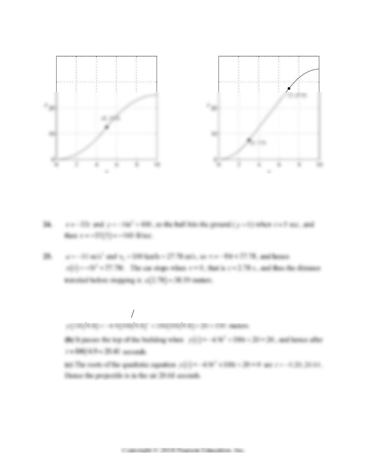
20. The graph of
vt shows that
if 0 5
5if 5 10
tt
vt t
, so that
x
x
x
x
21. The graph of
vt shows that
if 0 5
10 if 5 10
tt
vt tt
, so that
x
x
x
x
2
1
1
2
if 0 5
tC t
22. For 03t, 5
3
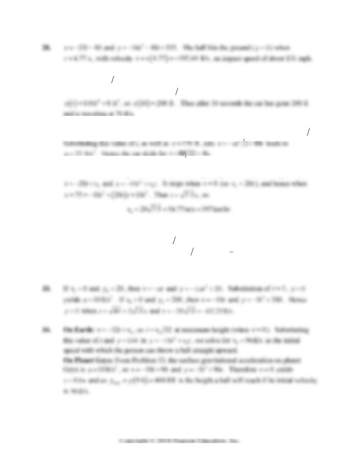
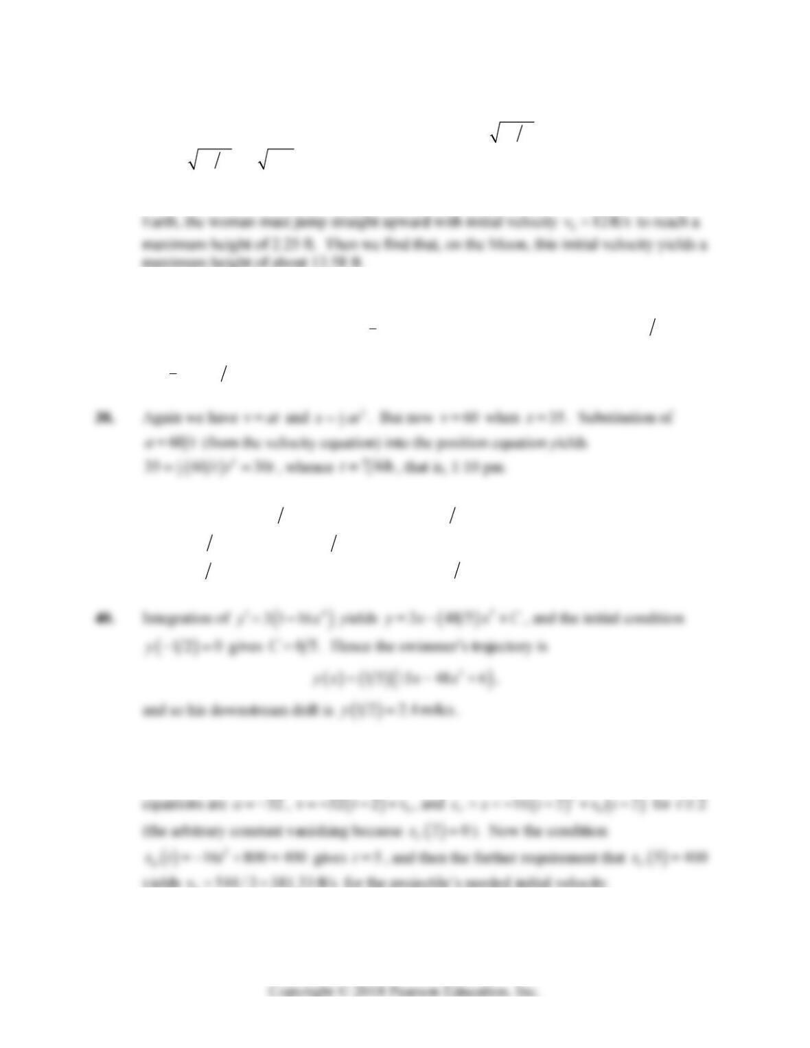
()vt t, so
2
5
1
6
x
ttC
. Now 10C because
00x, so
2
5
6
x
tt on this first interval, and its right-endpoint value is
15
2
3x.
x
x
x
30
40
Problem 19
30
40
Problem 20
12 Chapter 1: First-Order Differential Equations
23.
9.8 49vt t , so the ball reaches its maximum height ( 0v) after 5t seconds. Its
maximum height then is
2
5 4.9 5 49 5 122.5 metersy .
26. 9.8 100vt and 2
4.9 100 20ytt .
(a) 0v when 100 9.8 st, so the projectile’s maximum height is
27. 2
9.8 m/sa , so 9.8 10vt and 2
0
4.9 10ytty . The ball hits the ground
when 0y and 9.8 10 60 m/svt , so 5.10 st. Hence the height of the building
is
2
04.9 5.10 10 5.10 178.57 my
.
30
40
Problem 21
30
40
Problem 22
Section 1.2: Integrals as General and Particular Solutions 13
29. Integration of 2
0.12 0.6dv dt t t with
00v gives
32
0.04 0.3vt t t
. Hence
10 70 ft/sv. Then integration of 32
0.04 0.3dx dt t t with
00x gives
30. Taking 00x and 060 mph 88 ft/sv, we get 88vat , and 0v yields 88ta.
31. If 2
20 m/sa
and 00x, then the car’s velocity and position at time t are given by
x
32. Starting with 00x and 4
050 km/h 5 10 m/hv
, we find by the method of Problem
30 that the car’s deceleration is
72
25 3 10 m/ha
. Then, starting with 00x and
5
0100 km/h 10 m/hv
, we substitute 0
tva into 2
1
0
2
x
at v t and find that
60 mx when 0v. Thus doubling the initial velocity quadruples the distance the car
skids.
14 Chapter 1: First-Order Differential Equations
35. If
0
0v
and 0
y
h, then the stone’s velocity and height are given by vgt and
2
0.5
y
gt h , respectively. Hence 0y when 2thg, so
22vghg gh .
36. The method of solution is precisely the same as that in Problem 30. We find first that, on
37. We use units of miles and hours. If 00
0xv, then the car’s velocity and position after
t hours are given by
vat
and 2
1
2
x
at, respectively. Since 60v when 56t, the
velocity equation yields . Hence the distance traveled by 12:50 pm is
2
1
272 5 6 25 milesx .
x
39. Integration of
2
914
S
y
vx
yields
3
334
S
y
vxxC
, and the initial condi-
tion
12 0y
gives 3S
Cv. Hence the swimmers trajectory is
3
3341
S
yx v x x
. Substitution of
12 1y now gives 6mph
S
v.
y
41. The bomb equations are 32a , 32vt , and 2
16 800
B
ss t with 0t at the
instant the bomb is dropped. The projectile is fired at time 2,t so its corresponding