Section 7.3: The Eigenvalue Method for Linear Systems 395
35. Suppose 11 22 12 21
() () () () () 0.Wa x ax a x ax a Then the coefficient determinant of
the homogeneous linear system 111 212 121 2 22
() () 0, () () 0cxacxa cxacxa
vanishes. The system therefore has a non-trivial solution 12
{, }cc such that
36. The argument is precisely the same, except with n solution vectors each having n
component functions (rather than 2 solution vectors each having 2 component functions).
37. Suppose that 11 2 2
() () () .
nn
ctc t c t xx x0 Then the ith scalar component of this
SECTION 7.3
THE EIGENVALUE METHOD
FOR LINEAR SYSTEMS
In each of Problems 1–16 we give the characteristic equation, the eigenvalues
1 and
2 of the
coefficient matrix of the given system, the corresponding equations determining the associated
eigenvectors TT
111 2 22
[]and [ ],ab a bvv these eigenvectors, and the resulting scalar
components x1(t) and x2(t) of a general solution 12
11 2 2
() tt
tcece
xvv of the system.
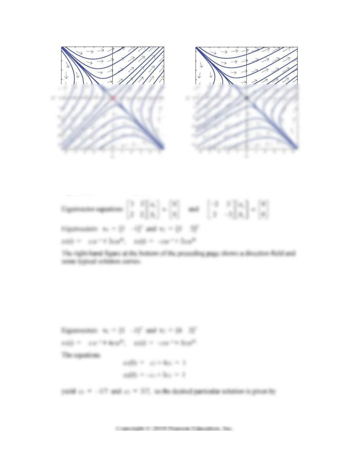
1. Characteristic equation 2230
Eigenvalues
1 = –1 and
2 = 3
396 Chapter 7: Linear Systems of Differential Equations
2
3
4
5
2
3
4
5
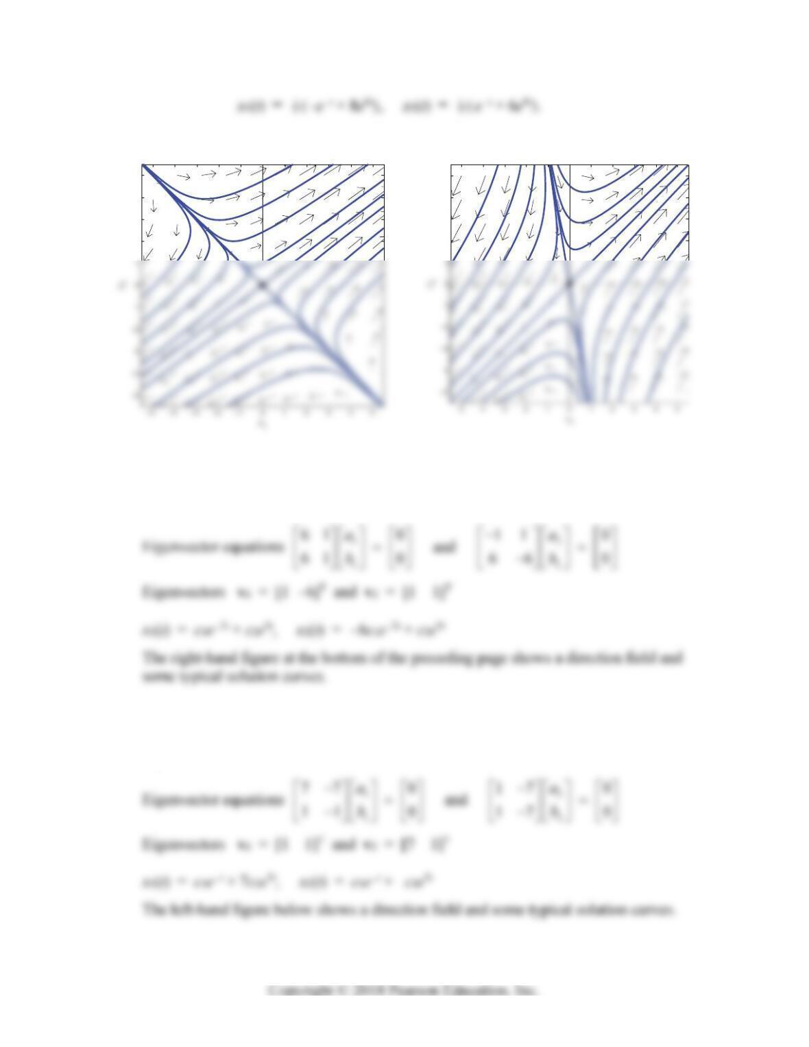
2. Characteristic equation 2340
Eigenvalues
1 = –1 and
2 = 4
3. Characteristic equation 2560
Eigenvalues
1 = –1 and
2 = 6
Eigenvector equations 12
12
44 0 3 4 0
and
33 0 3 4 0
aa
bb
Section 7.3: The Eigenvalue Method for Linear Systems 397
2
3
4
5
2
3
4
5
The left-hand figure below shows a direction field and some typical solution curves.
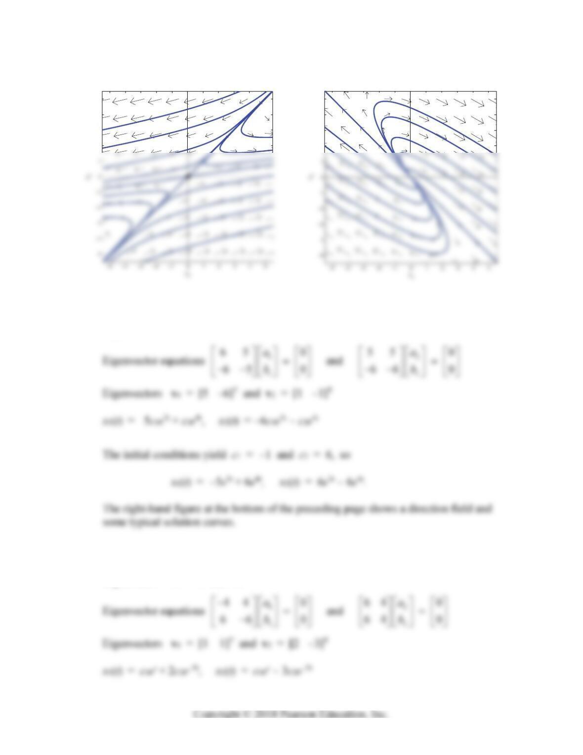
4. Characteristic equation 2310 0
Eigenvalues
1 = –2 and
2 = 5
5. Characteristic equation 2450
Eigenvalues
1 = –1 and
2 = 5
398 Chapter 7: Linear Systems of Differential Equations
2
3
4
5
2
3
4
5
6. Characteristic equation 27120
Eigenvalues
1 = 3 and
2 = 4
7. Characteristic equation 2890
Eigenvalues
1 = 1 and
2 = –9
Section 7.3: The Eigenvalue Method for Linear Systems 399
3
4
5
x
1
3
4
5
1
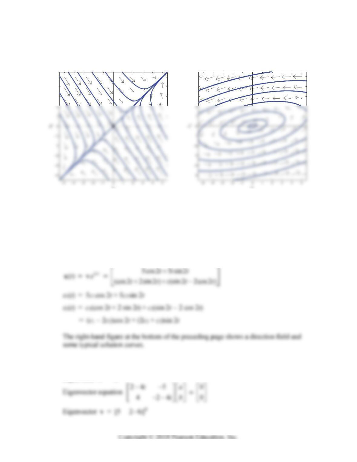
The left-hand figure below shows a direction field and some typical solution curves.
8. Characteristic equation
2 + 4 = 0
Eigenvalue
= 2i
Eigenvector equation 12 5 0
112 0
ia
ib
Eigenvector v = [5 1–2i]T
9. Characteristic equation
2 + 16 = 0
Eigenvalue
= 4i
400 Chapter 7: Linear Systems of Differential Equations
2
3
4
5
2
3
4
5
The real and imaginary parts of
45cos4 5 sin4
() (2cos4 4sin4 ) (2sin4 4cos4 )
it ti t
te
ttit t
xv
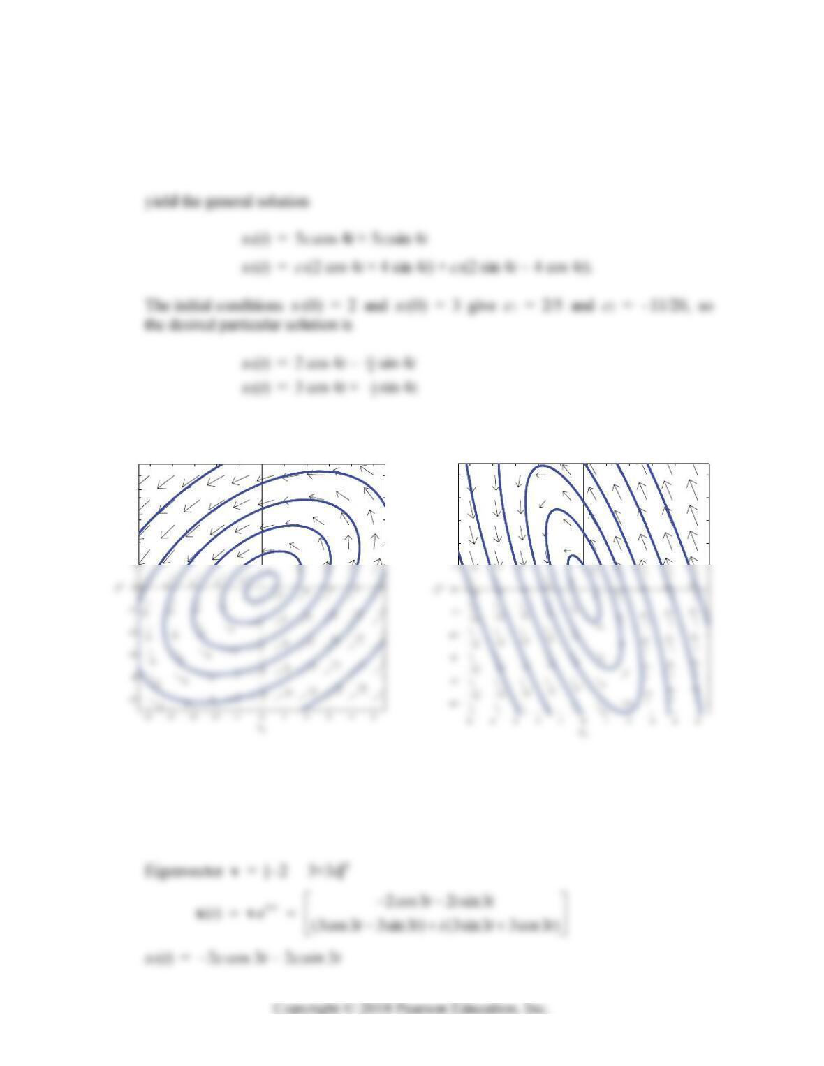
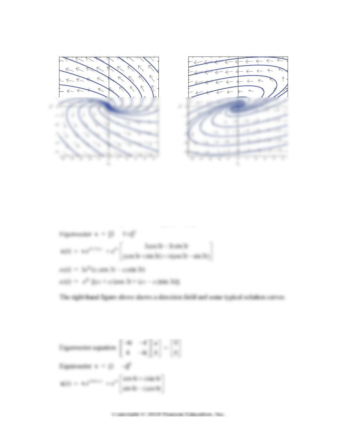
The left-hand figure at the top of the next page shows a direction field and some typical
solution curves.
10. Characteristic equation
2 + 9 = 0
Eigenvalue
= 3i
Eigenvector equation 33 2 0
933 0
ia
ib
Section 7.3: The Eigenvalue Method for Linear Systems 401
11. Characteristic equation 2250
Eigenvalue
= 1 – 2i
Eigenvector equation 22 0
22 0
ia
ib
Eigenvector v = [1 i]T
402 Chapter 7: Linear Systems of Differential Equations
2
3
4
5
x
1
12. Characteristic equation
2 – 4
+ 8 = 0
Eigenvalue
= 2 + 2i
Eigenvector equation 12 5 0
112 0
ia
ib
Section 7.3: The Eigenvalue Method for Linear Systems 403
2
3
4
5
2
3
4
5
13. Characteristic equation
2 – 4
+ 13 = 0
Eigenvalue
= 2 – 3i
Eigenvector equation 33 9 0
233 0
ia
ib
14. Characteristic equation 2250
Eigenvalue
= 3 + 4i
404 Chapter 7: Linear Systems of Differential Equations
x1(t) = e3t(c1cos 4t + c2sin 4t)
x2(t) = e3t(c1sin 4t – c2cos 4t)
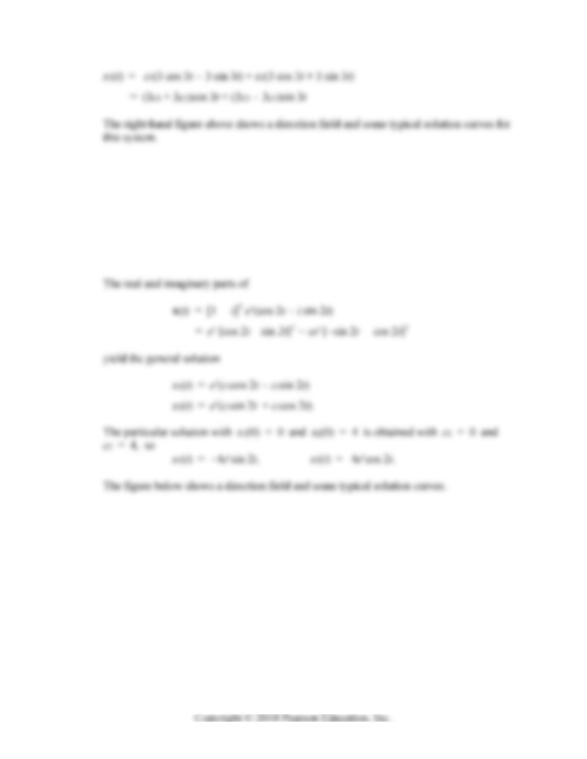
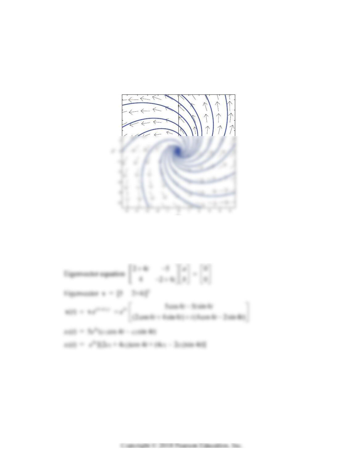
The figure below shows a direction field and some typical solution curves.
2
3
4
5
x
1
15. Characteristic equation
2 – 10
+ 41 = 0
Eigenvalue
= 5 – 4i
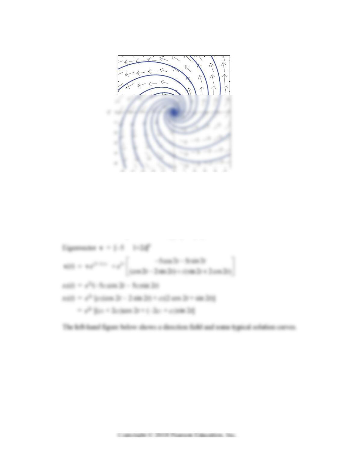
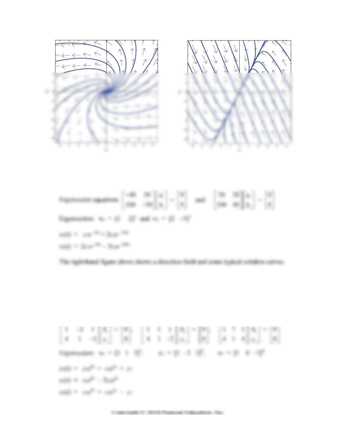
The left-hand figure at the top of the next page shows a direction field and some typical
solution curves.
Section 7.3: The Eigenvalue Method for Linear Systems 405
3
4
5
1
16. Characteristic equation
2 + 110
+1000 = 0
Eigenvalues
1 = –10 and
2 = –100
17. Characteristic equation 32
15 54 0
Eigenvalues
1 = 9,
2 = 6,
3 = 0
Eigenvector equations
123
51 4 0 214 0 414 0
aaa
3
4
5
1
406 Chapter 7: Linear Systems of Differential Equations
18. Characteristic equation 32
15 54 0
Eigenvalues
1 = 9,
2 = 6,
3 = 0
Eigenvector equations
123
82 2 0 522 0 122 0
aaa
19. Characteristic equation 32
12 45 54 0
Eigenvalues
1 = 6,
2 = 3,
3 = 3
Eigenvector equations
123
2 1 1 0 111 0 111 0
aa a
20. Characteristic equation 32
17 84 108 0
Eigenvalues
1 = 9,
2 = 6,
3 = 2
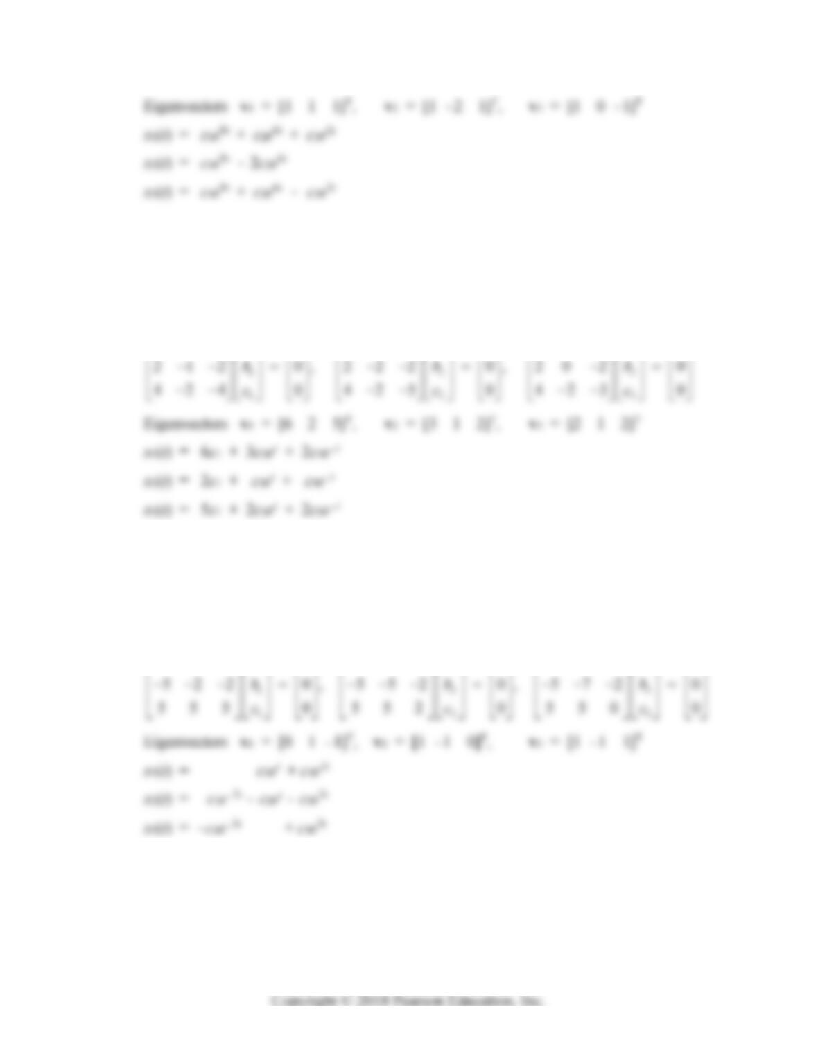
Eigenvector equations
123
41 3 0 113 0 313 0
aaa
Section 7.3: The Eigenvalue Method for Linear Systems 407
21. Characteristic equation 30
Eigenvalues
1 = 0,
2 = 1,
3 = –1
Eigenvector equations
123
50 6 0 40 6 0 60 6 0
aa a
22. Characteristic equation 32
2560
Distinct eigenvalues
1 = – 2,
2 = 1,
3 = 3
Eigenvector equations
12 3
522 0 222 0 022 0
aa a
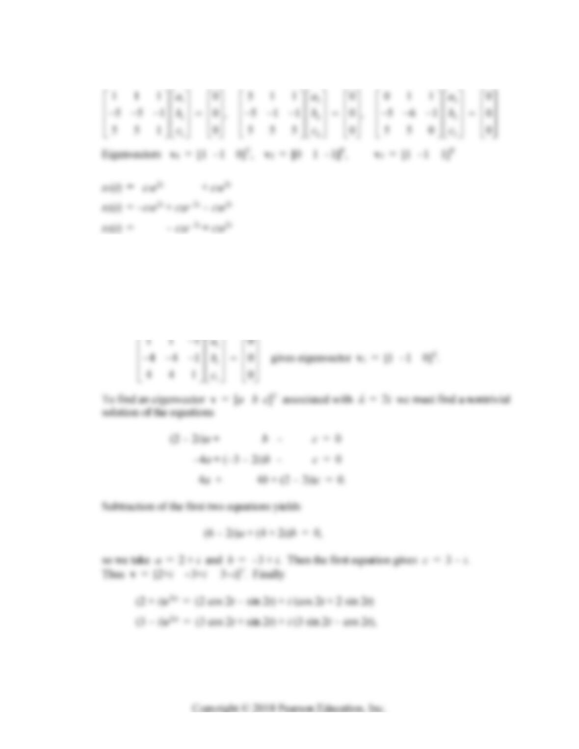
23. Characteristic equation 32
34120
Eigenvalues
1 = 2,
2 = –2,
3 = 3
408 Chapter 7: Linear Systems of Differential Equations
Eigenvector equations
24. Characteristic equation 32
440
Eigenvalues
= 1 and
= ±2i
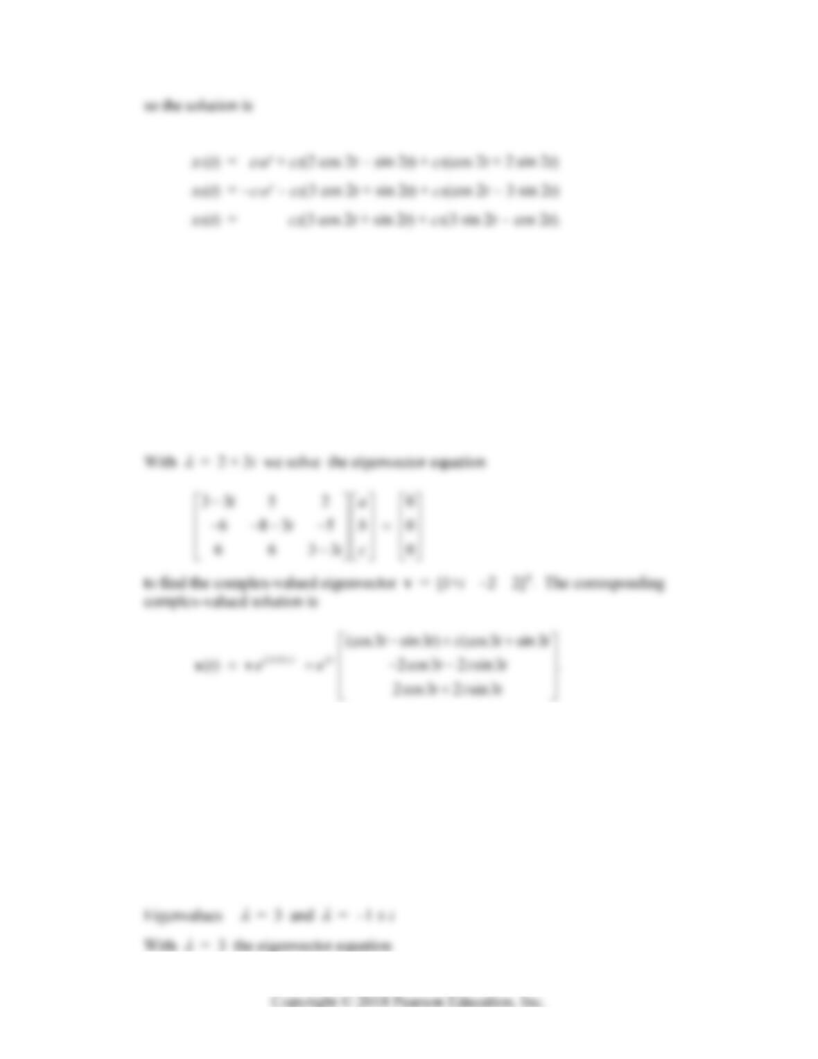
With
= 1 the eigenvector equation
Section 7.3: The Eigenvalue Method for Linear Systems 409
25. Characteristic equation 32
413 0
Eigenvalues = 0 and 2 ± 3i
With
= 1 the eigenvector equation
1
1
1
552 0
665 0
665 0
a
b
c
gives eigenvector v1 = [1 –1 0]T.
The scalar components of the resulting general solution are
x1(t) = c1 + e2t [(c2 + c3)cos 3t + (–c2 + c3)sin 3t]
x2(t) = –c1 + 2e2t(–c2cos 3t – c3sin 3t)
x3(t) = 2e2t(c2cos 3t + c3sin 3t)
26. Characteristic equation 32
460
410 Chapter 7: Linear Systems of Differential Equations
1
1
1
001 0
942 0
94 4 0
a
b
c
gives eigenvector v1 = [4 9 0]T.
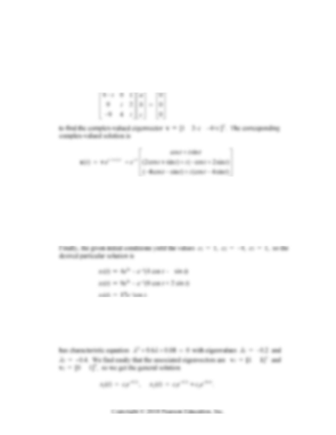
With
= –1 + i we solve the eigenvector equation
with real and imaginary parts x2(t) and x3(t). Assembling the general solution
x = c1x1 + c2x2 +c3x3, we get the scalar equations
x1(t) = 4c1e3t + e–t [c2cos t + c3sin t]
x2(t) = 9c1e3t + e–t [(2c2 – c3)cos t + (c2 + 2c3)sin t]
x3(t) = e–t [(–4c2 + c3)cos t + (–c2 – 4c3)sin t].
27. The coefficient matrix
0.2 0
0.2 0.4
A
Section 7.3: The Eigenvalue Method for Linear Systems 411
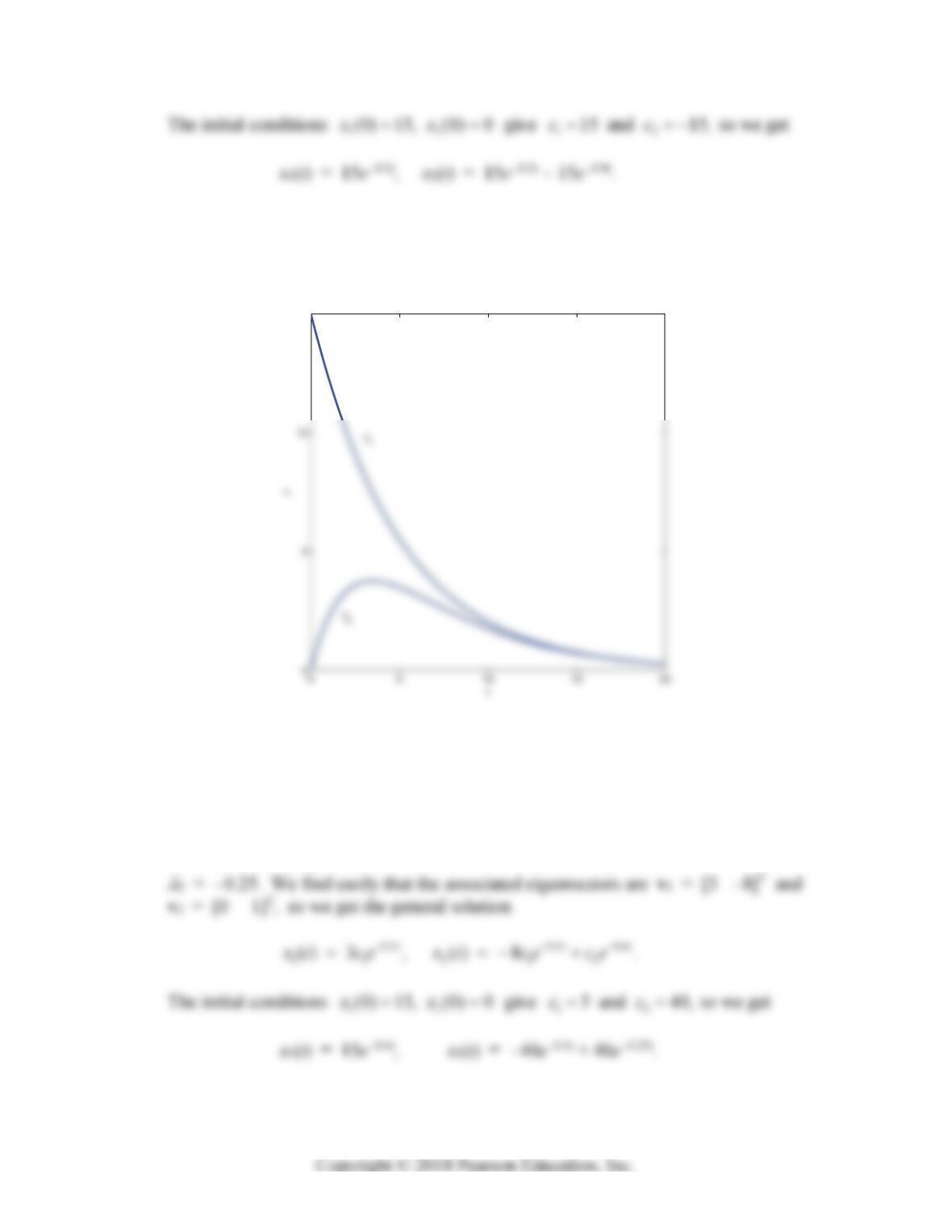
To find the maximum value of x2(t), we solve the equation 2() 0xt
for t = 5 ln 2,
which gives the maximum value x2(5 ln 2) = 3.75 lb. The following figure shows the
graphs of 12
() and ().
x
txt
15
28. The coefficient matrix
0.4 0
0.4 0.25
A
has characteristic equation 20.65 0.10 0
with eigenvalues
1 = –0.4 and
412 Chapter 7: Linear Systems of Differential Equations
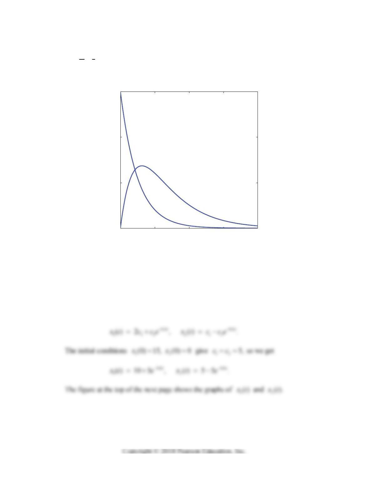
To find the maximum value of x2(t), we solve the equation 2() 0xt
for
tm = 20 8
35
ln , which gives the maximum value 2( ) 6.85
m
xt lb. The following figure
shows the graphs of 12
() and ().
x
txt
0 5 10 15 20
0
5
10
15
t
x
x1
x2
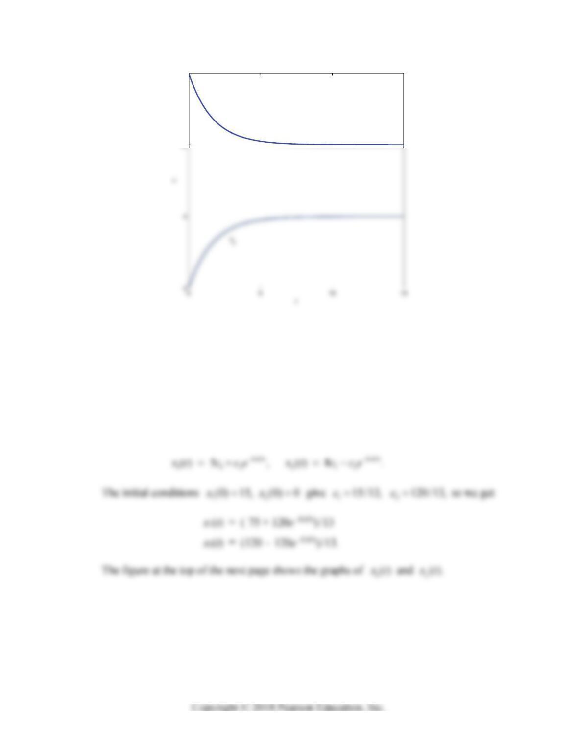
29. The coefficient matrix
0.2 0.4
0.2 0.4
A
has eigenvalues
1 = 0 and
2 = –0.6, with eigenvectors v1 = [2 1]T and
v2 = [1 –1]T that yield the general solution
x
Section 7.3: The Eigenvalue Method for Linear Systems 413
10
15
x
1
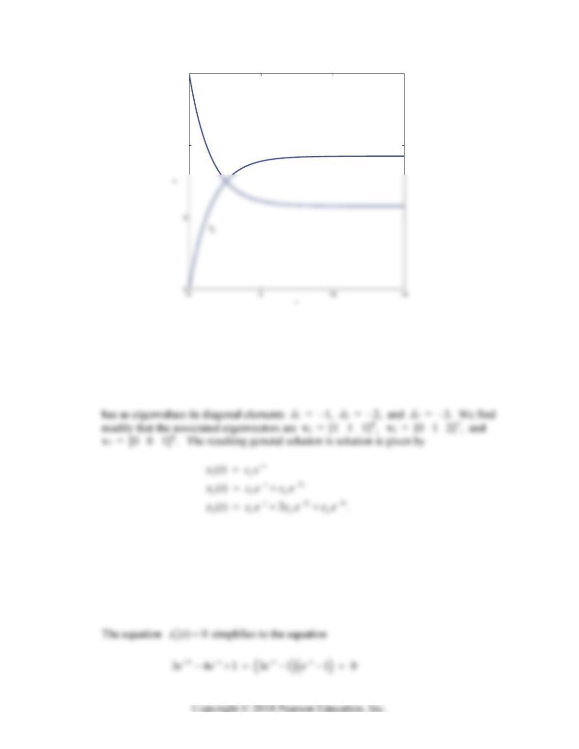
30. The coefficient matrix
0.4 0.25
0.4 0.25
A
has eigenvalues
1 = 0 and
2 = –0.65, with eigenvectors v1 = [5 8]T and
v2 = [1 –1]T that yield the general solution
414 Chapter 7: Linear Systems of Differential Equations
10
15
x
1
31. The coefficient matrix
10 0
120
02 3
A
x
The initial conditions 122
(0) 27, (0) (0) 0xxx give 13 2
27, 27,cc c so we
get
1
2
2
23
3
() 27
( ) 27 27
( ) 27 54 27 .
t
tt
ttt
xt e
xt e e
x
teee