Section 10.2: Transformation of Initial Value Problems 575
2
22
11
() (1)( 1) 1
ss
Xs ss s
Hence the solution is
x(t) = cos t + sin t
y(t) = et – cos t
z(t) = –2 sin t.
17.
33 3
00
11
() 1
33
t
tt
ft e d e e
21.
00
00
sin (1 cos ) sin sin
()
t
t
ttdt d t t
ft d
22.
1
3
00
11
sinh 3 cosh 3 cosh 3 1
() 99
t
tt
ft d
576 Chapter 10: Laplace Transform Methods
26. With f(t) = sinh kt and F(s) = k/(s2 – k2), Theorem 1 yields
L{f
(t)} = L{k cosh kt} = ks/(s2 – k2) = sF(s),
so it follows upon division by k that L{cosh kt} = s/(s2 – k2).
27. (a) With f(t) = tneat and f
(t) = ntn–1eat + atneat, Theorem 1 yields
(b)
2
1111
1: ()
at at
nte e
sa sasa sa
LL
28. Problems 28 and 30 are the trigonometric and hyperbolic versions of essentially the same
computation. For Problem 30 we let f(t) = t cosh kt, so f(0) = 0. Then
()
f
t
= cosh kt + kt sinh kt
()
f
t
= 2k sinh kt + k2t cosh kt,
Section 10.2: Transformation of Initial Value Problems 577
29. Let f(t) = t sinh kt, so f(0) = 0. Then
()
f
t
= sinh kt + kt cosh kt
()
f
t
= 2k cosh kt + k2t sinh kt,
30. See Problem 28.
31. Using the known transform of sin kt and the Problem 28 transform of t cos kt, we obtain
32. If f(t) = u(t – a), then the only jump in f(t) is j1 = 1 at t1 = a. Since f(0) = 0 and
f
(t) = 0, Formula (21) in this section yields
578 Chapter 10: Laplace Transform Methods
33. () () () ( ) ( ),
ab
f
tutututautbso the result of Problem 32 gives
34. The square wave function of Figure 10.2.9 has a sequence {tn} of jumps with tn = n
and jn = 2(–1)n for n = 1, 2, 3, … . Hence Formula (21) yields
0 = s F(s) – 1 –
1
2( 1) .
ns n
n
e
It follows that
35. Let’s write ( )gt for the on-off function of this problem to distinguish it from the square
wave function of Problem 34. Then comparison of Figures 10.2.9 and 10.2.10 makes it
clear that
1
2
() 1 () ,gt f t so (using the result of Problem 34) we obtain
36. If g(t) is the triangular wave function of Figure 10.2.11 and f(t) is the square wave
function of Problem 34, then () ().gt ft
Hence Theorem 1 and the result of Problem
Section 10.3: Translation and Partial Fractions 579
37. We observe that (0) 0f and that the sawtooth function has jump –1 at each of the
points 1, 2, 3, .
n
tn Also, () 1ft
wherever the derivative is defined. Hence
Eq. (22) in this section gives
SECTION 10.3
TRANSLATION AND PARTIAL FRACTIONS
This section is devoted to the computational nuts and bolts of the staple technique for the
inversion of Laplace transforms — partial fraction decompositions. If time does not permit
going further in this chapter, Sections 10.1–10.3 provide a self-contained introduction to Laplace
transforms that suffices for the most common elementary applications.
1. L{t4} = 5
24
s, so L{t4e
t} = 5
24
()s
2. L{t3/2} = 5/2
3,
4s
so L{t3/2 e–4t} = 5/2
3.
4( 4)s
5. 2
331 3
() ,so ()
24 2 2 2
t
Fs ft e
ss
580 Chapter 10: Laplace Transform Methods
6.
22
323
(1)2 1 2
() ,so ()
(1) (1) (1)
ttt
s
Fs ft te te e t t
sss
10.
22
23 1 23
() 9
32 16 2/3 16/9
ss
Fs ss
22 22
22/354/3
936
2/3 4/3 2/3 4/3
s
ss
2/3
144
() 8cos 5sin
36 3 3
ttt
ft e
14. 2
111
() 2 3 , so () 2 3
12
tt
Fs ft e e
ss s
15.
5
2
1111 1
() 1 5 , so () 1 5
25 5 25
t
Fs ft t e
sss
Section 10.3: Translation and Partial Fractions 581
17. 22 22
11 1 1 2 2
() 84 4164 4
Fs ss ss
1
() sinh2 sin2
16
f
ttt
f
f
20.
222 2 2
2
1111212
() 32 2 2
22 2 2
4
Fs ss
ss s s
s
22
1
() 12 12
32
tt
f
tetet
21. First we need to find , , ,ABCD so that
which we solve for 0, 1, 2, 1.ABC D Thus
582 Chapter 10: Laplace Transform Methods
22. First we need to find A, B, C, D so that
32
22
2
22
2.
445
445 445
ss AsB CsD
ss
ss ss
When we multiply each side by 22
(4 4 5)ss we get the identity
it follows that
11
22
22
2
11
22
13 4
11
() .
832
11
ss
Fs ss
Finally the results
23.
3
44 2 22 2
1,
4222 22
ssasa
sa sasasasa
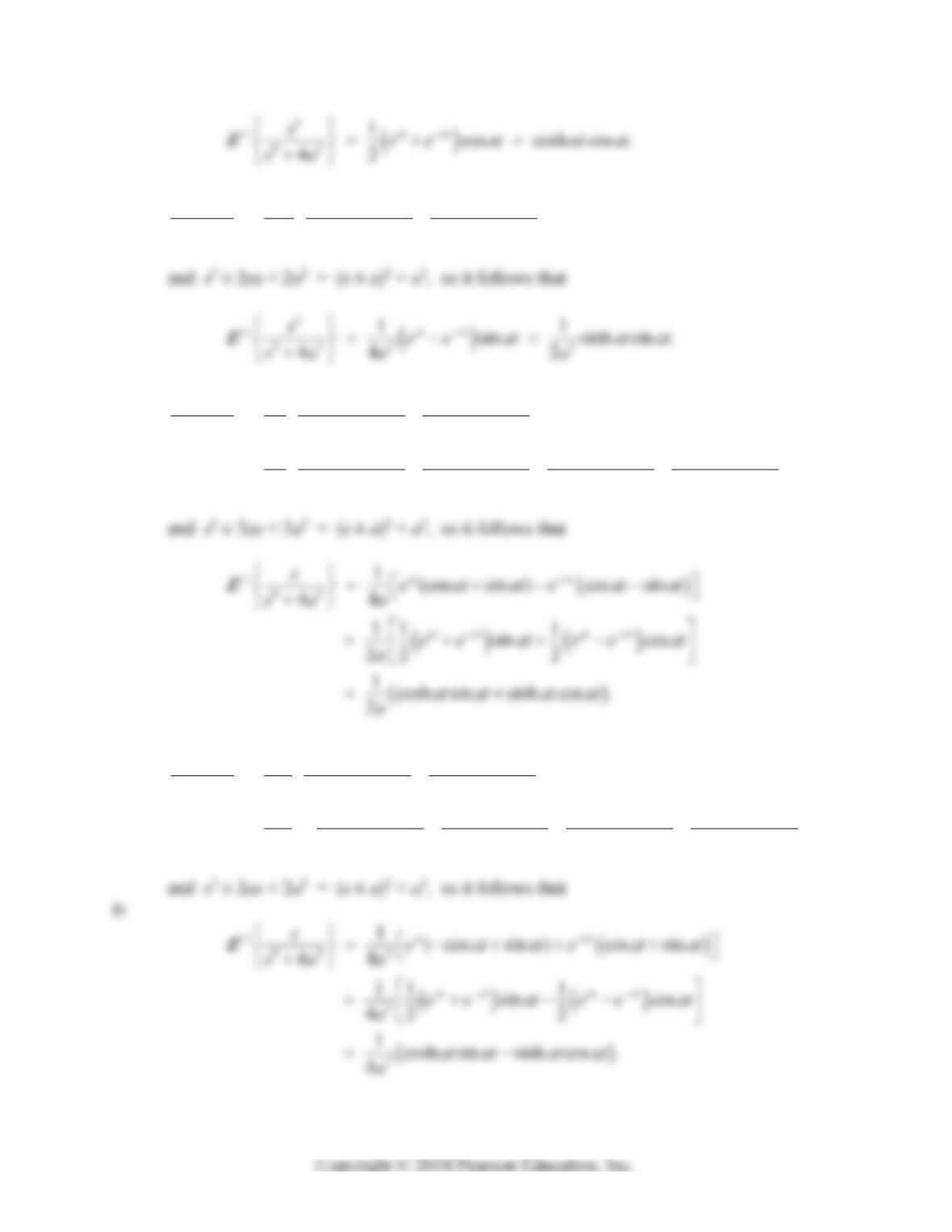
and s2 ± 2as + 2a2 = (s ± a)2 + a2, so it follows that
Section 10.3: Translation and Partial Fractions 583
24. 44 22 22 2
1,
4 4 22 22
saa
s a a s as a s as a
25. 44 2 22 2
1
4 4 22 22
sss
s a a s as a s as a
22222222
1,
422222222
sa a sa a
a s as a s as a s as a s as a
26. 44 32 22 2
11 2 2
4 8 22 22
sa sa
s a a s as a s as a
3 2 22 22 22 2
1,
822222222
sa a sa a
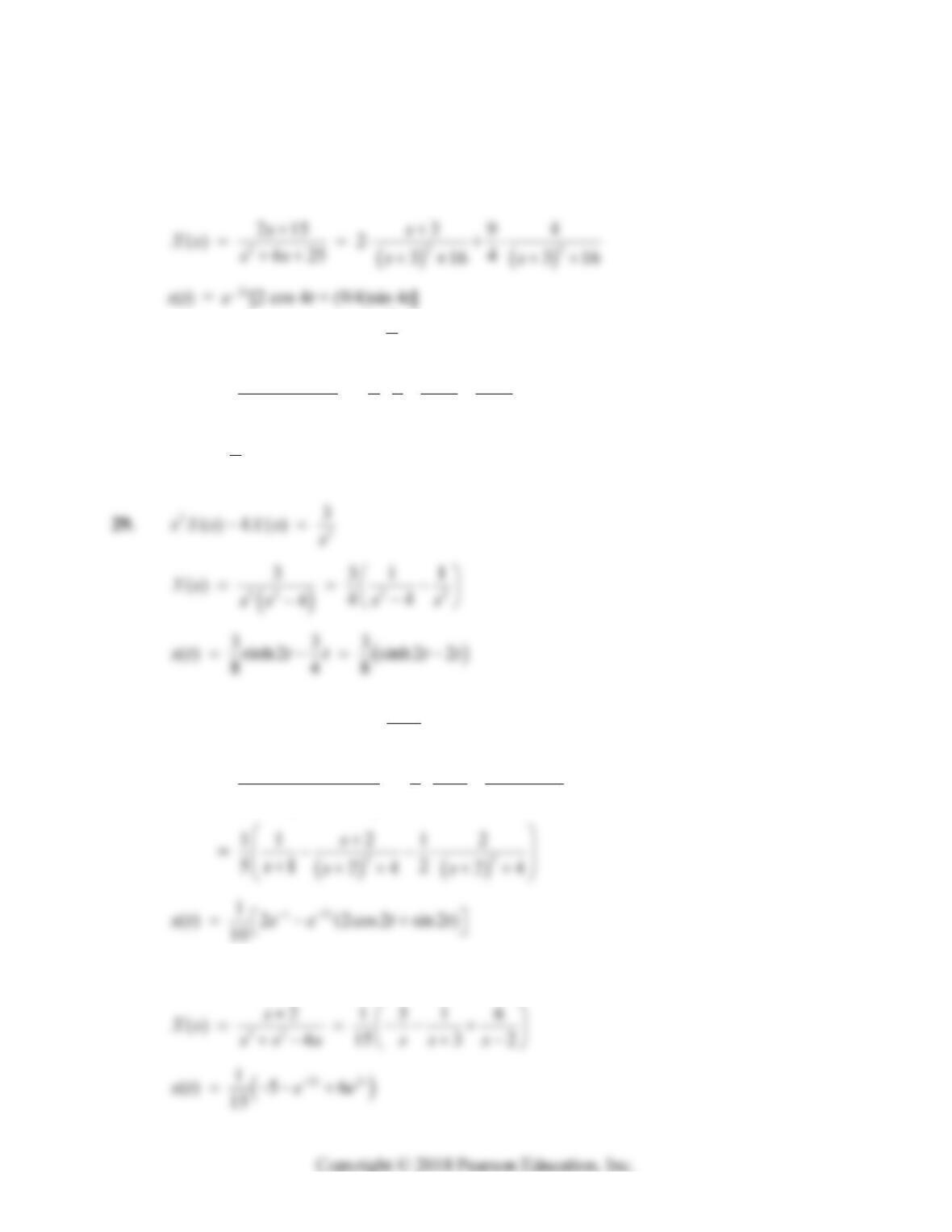
a s as a s as a s as a s as a
584 Chapter 10: Laplace Transform Methods
In Problems 27–40 we give first the transformed equation, then the Laplace transform ( )
X
s of
the solution, and finally the desired solution ( ).
x
t
27. [s2X(s) – 2s – 3] + 6[sX(s) – 2] + 25X(s) = 0
28. 22
() 6 () 8 ()sXs sXs Xs s
2
21112
() (68)4 4 2
Xs ss s s s s
42
1
() 1 2
4
tt
x
tee
x
30. 21
() 4 () 8 () 1
sXs sXs Xs s
x
2
2
1113
() 51 48
148
s
Xs sss
sss
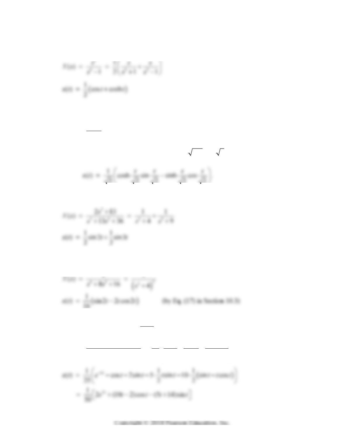
31. [s3X(s) – s – 1] + [s2X(s) – 1] – 6[sX(s)] = 0
Section 10.3: Translation and Partial Fractions 585
32. 43
() () 0sXs s Xs
33. [s4X(s) – 1] + X(s) = 0
4
1
() 1
Xs s
It therefore follows from Problem 26 with 41/4 1/ 2a that
222 22
34. [s4X(s) – 2s2 + 13] + 13[s2X(s) – 2] + 36 X(s) = 0
35. 42
() 1 8 () 16 () 0sXs sXs Xs
36. 42 1
() 2 () () 2
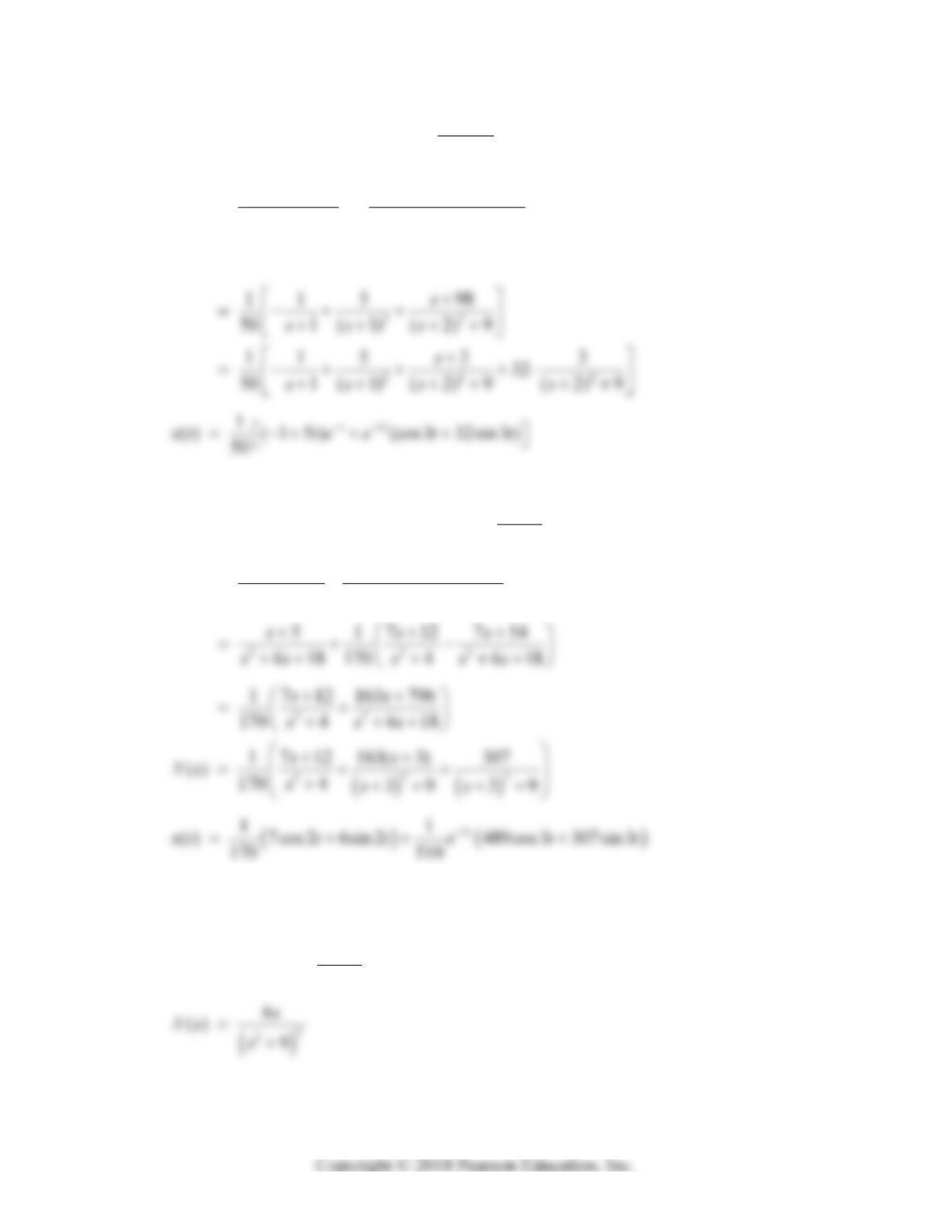
sXs sXs Xs s
2
2
42 2
11125(2)
() 25 2 1
221 1
ss
Xs ss
sss s
586 Chapter 10: Laplace Transform Methods
37.
2
2
1
() 2 4 () 13 () 1
sXs sXs Xs s
22
222
21/( 1) 2 4 3
() 413 (1) 413
sss
Xs ss sss
38.
2
2
() 1 6 () 1 18 () 4
s
sXs s sXs Xs s
222
5
() 618 4618
ss
Xs ss sss
39. 96cos3,(0)(0)0xx tx x
2
2
6
() 9 () 9
s
sXs Xs s
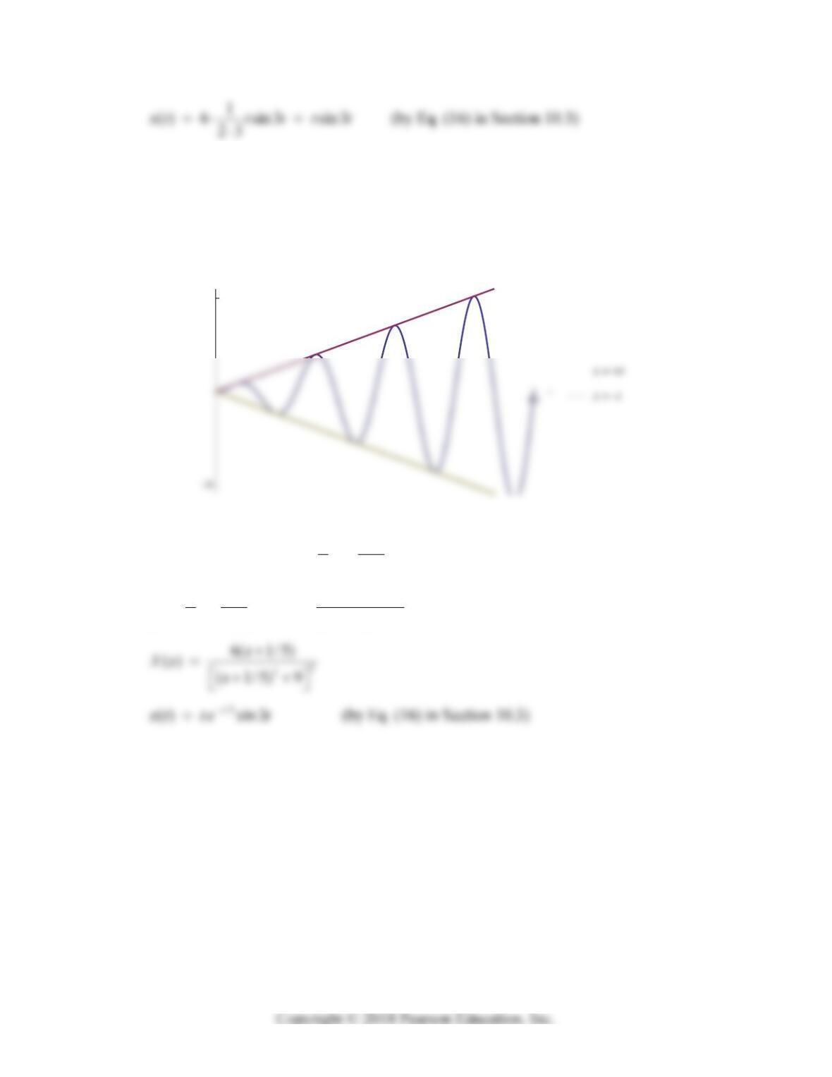
Section 10.3: Translation and Partial Fractions 587
x
The graph of this resonance is shown in the figure at the top of the next page.
20
x
40. /5
2226
0.4 9.04 6 cos3
525
t
x
xxxx e t
2
2
2226 6(1/5)
()
525 (1/5)9
s
ss Xs s
x
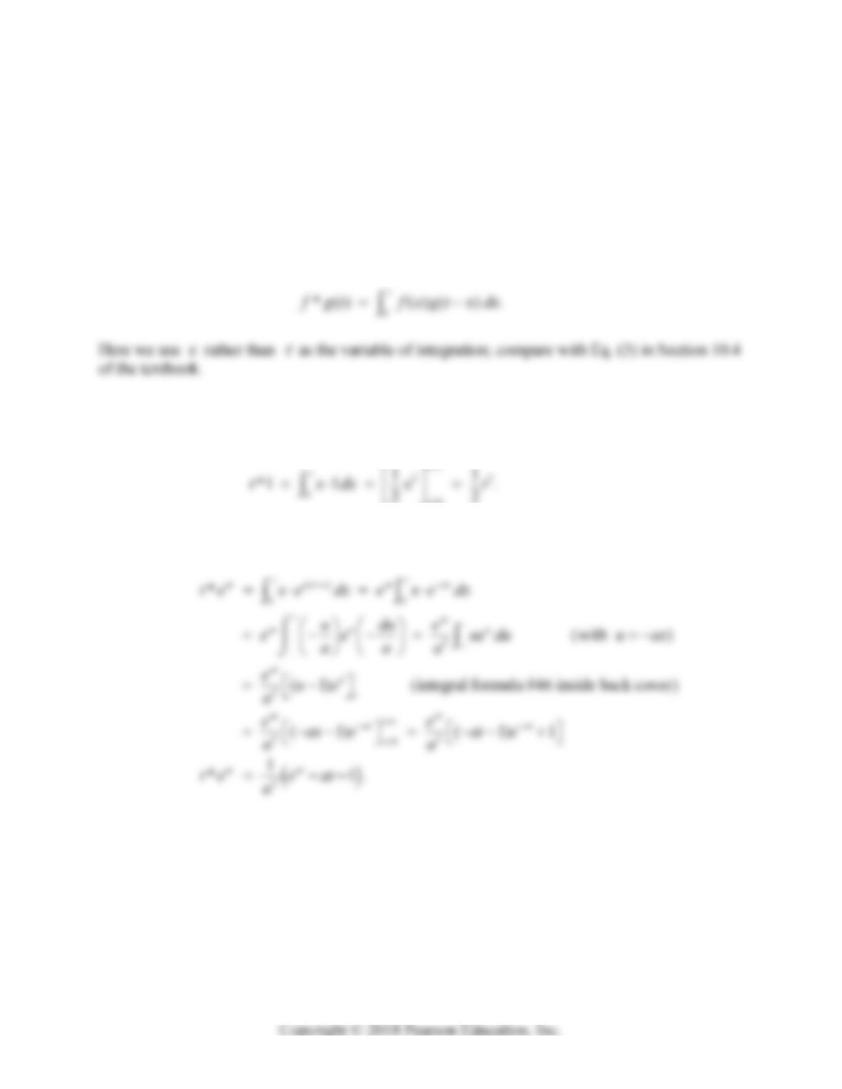
588 Chapter 10: Laplace Transform Methods
SECTION 10.4
DERIVATIVES, INTEGRALS, AND
PRODUCTS OF TRANSFORMS
This section completes the presentation of the standard “operational properties” of Laplace
transforms, the most important one here being the convolution property L{f*g} = L{f}L{g},
where the convolution f*g is defined by
1. With () and () 1ft t gt we calculate
x
2. With ( ) and ( ) at
f
tt gte we calculate
3. To compute 0
(sin ) * (sin ) sin sin( ) ,
t
tt xtxdx
we first apply the identity
sin A sin B = [cos(A – B) – cos(A + B)]/2. This gives
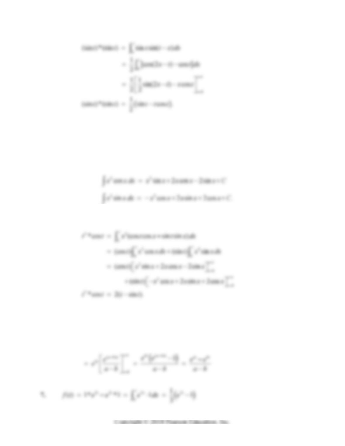
Section 10.4: Derivatives, Integrals, and Products of Transforms 589
4. To compute 22
0
*cos cos( ) ,
t
ttxtxdx
we first substitute
cos(t – x) = cos t cos x + sin t sin x,
and then use the integral formulas
from #40 and #41 inside the back cover of the textbook. This gives
5.
()
0
00
*tt
xt
at at ax a t x at at at
x
ee ee dx edx ex te
6. () ( )
00
*tt
at bt ax b t x bt a b x
e e e e dx e e dx
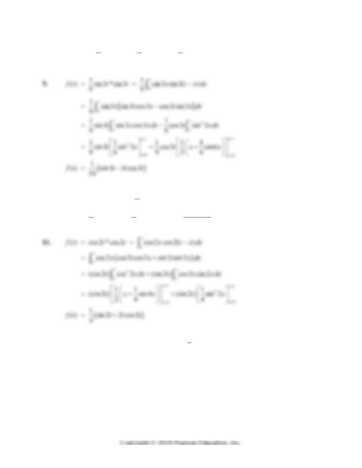
590 Chapter 10: Laplace Transform Methods
8.
0
111
( ) 1* sin 2 sin 2 1 cos 2
224
t
f
ttxdx t
f
10. 0
1
() *(sin )/ sin ( )
t
f
tt ktk kxtxdx
k
3
00
1sin
sin sin
tt
tktkt
kx dx x kx dx
kk k
12. f(t) = (e–2tsin t)*(1) 22
0
1
sin 1 (cos 2sin )
5
txt
exdx e t t
Section 10.4: Derivatives, Integrals, and Products of Transforms 591
f
14. 0
( ) cos2 *sin cos2 sin( )
t
f
ttt xtxdx
0
00
cos2 (sin cos cos sin )
(sin ) cos 2 cos cos cos 2 sin
t
tt
xtx txdx
txxdxt xxdx
00
11
(sin ) cos3 cos cos sin 3 sin
22
1
() cos cos2
3
tt
txxdxtxxdx
ft t t
17. L{e2tcos 3t} = (s – 2)/(s2 – 4s + 13)
L{te2tcos 3t} = –(d/ds)[(s – 2)/(s2 – 4s + 13)] = (s2 – 4s – 5)/(s2 – 4s + 13)2
592 Chapter 10: Laplace Transform Methods
20.
2
1
1cos2 ,so
4
s
tss
L
21.
311
1,so
3
t
ess
L
23.
11 22
111112sinh2
() ( ) 22
tt t
ft F s e e
ttsst t
LL
24.
11
22
11222
( ) ( ) cos2 cos
14
ss
f
tFs tt
ttsst
LL
f
Section 10.4: Derivatives, Integrals, and Products of Transforms 593
28. An empirical approach works best with this one. We can construct transforms with
powers of (s2 + 1) in their denominators by differentiating the transforms of sin t and
cos t. Thus,
From the first and last of these formulas it follows readily that
29. –[s2X(s) – x(0)] – [s X(s)] – 2[s X(s)] + X(s) = 0
s(s + 1)X’(s) + 4s X(s) = 0 (separable)
X(s) = 4
(1)
A
s with A 0
x(t) = Ct3e–t with C 0
594 Chapter 10: Laplace Transform Methods
31. –[s2X(s) – x’(0)] + 4[s X(s)] – [s X(s)] –4[X(s)] + 2X(s) = 0
(s2 – 4s + 4)X’(s)+(3s – 6)X(s) = 0 (separable)
32. –[s2X(s) – x’(0)] – 2[s X(s)] – 2[s X(s)] – 2X(s) = 0
–(s2 + 2s)X’ (s) – (4s + 4)X(s) = 0 (separable)
33. –[s2X(s) – x(0)] – 2[s X(s)] – [X(s)] = 0
34. –(s2 + 4s + 13)X’(s) – (4s + 8)X(s) = 0
X(s) = 2
22 2
(413) (2)9
CC
ss s
It now follows from Problem 31 in Section 10.2 that