V = V0 + ∆V (1–e–ax)
Problem 4.2
The surface velocity of a river is measured at several locations x and can be reasonably
represented by
0(1 )
ax
VV V e
−
=+Δ − ,
where 0
V
, V
Δ
, and
a
are constants. Find the Lagrangian description of the velocity of a
fluid particle flowing along the surface if 0x= at time =0t.
Solution 4.2
GIVEN: See sketch.
FIND: 0
(,)VV t since we want the velocity of a fluid
particle (Lagrangian description).
SOLUTION: The position x is found from
Substituting the limits gives
Using the original equation for
V
gives
Substituting these expressions for ax
e− and x into Eq. (1) gives
or
Problem 4.3
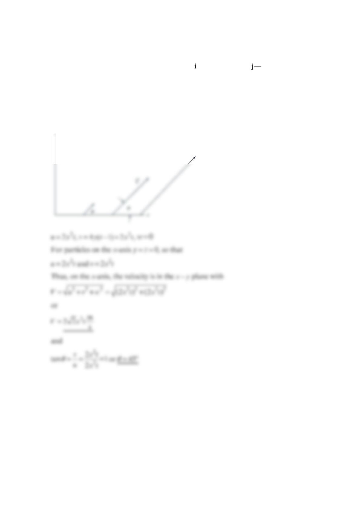
The velocity field of a flow is given by 22
m
2[4(1)2]
s
xt yt xt=+−+
V where x and
y
are in
meters and
t
is in seconds. For fluid particles on the x axis, determine the speed and
direction of flow.
Solution 4.3
y
Problem 4.4
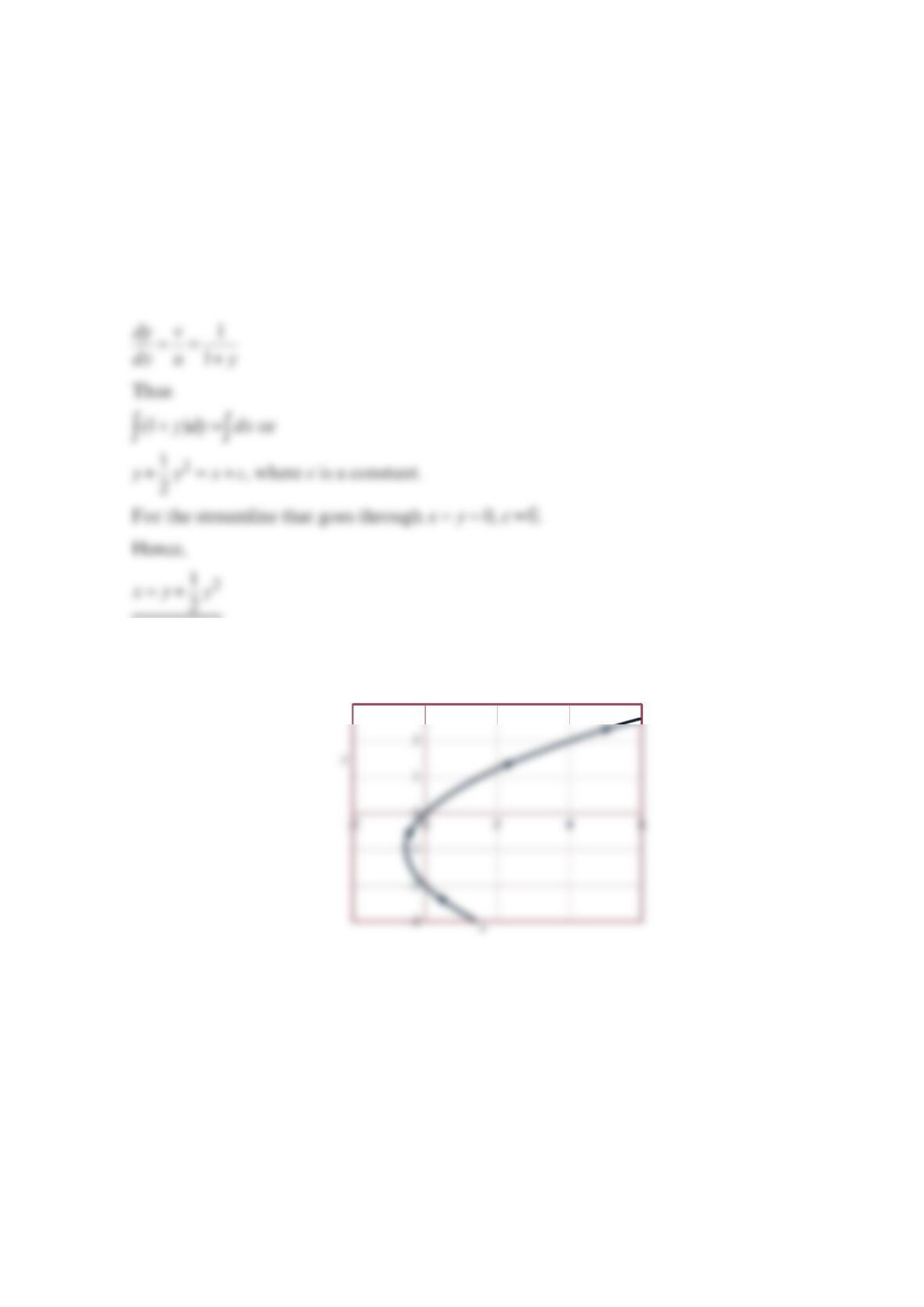
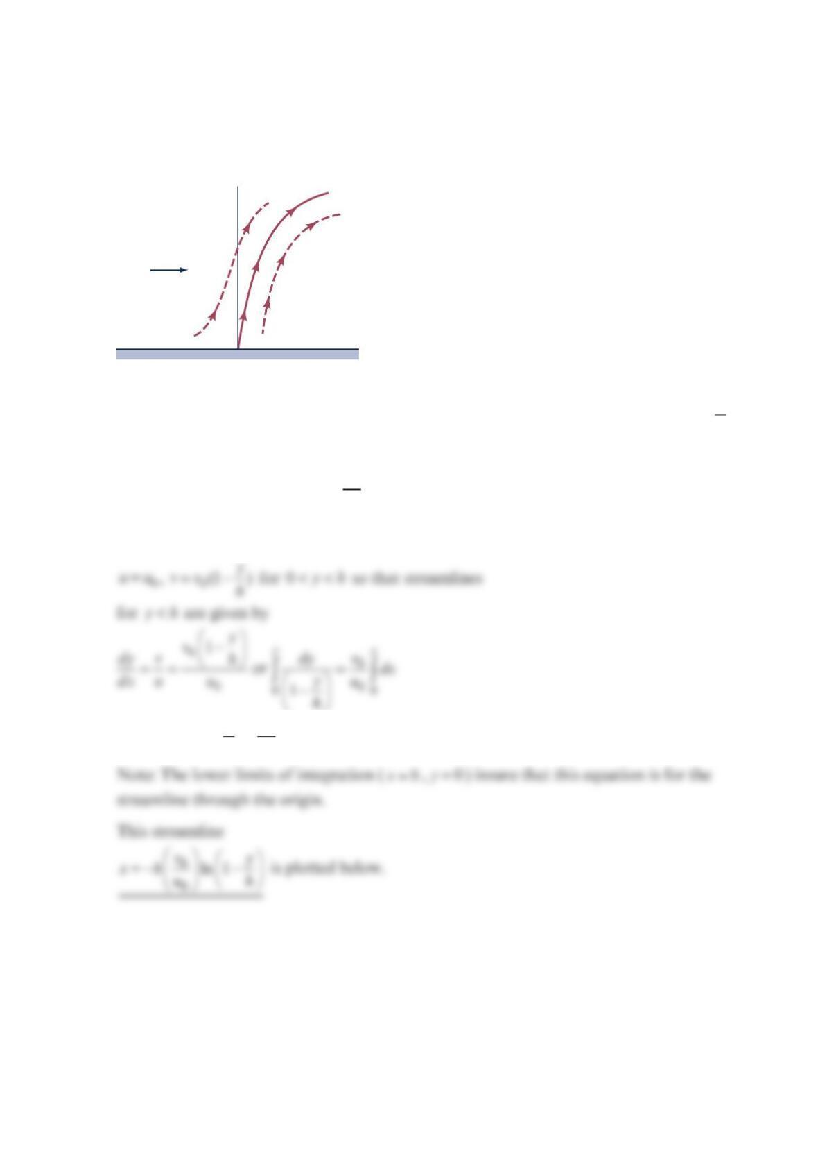
A two-dimensional velocity field is given by 1uy=+ and v = 1. Determine the equation of
the streamline that passes through the origin. On a graph, plot this streamline.
Solution 4.4
1uy=+ and 1v= so the streamlines are given by
This streamline is plotted below. Note that since 10v=>, the direction of flow is as
shown.
3
Problem 4.5
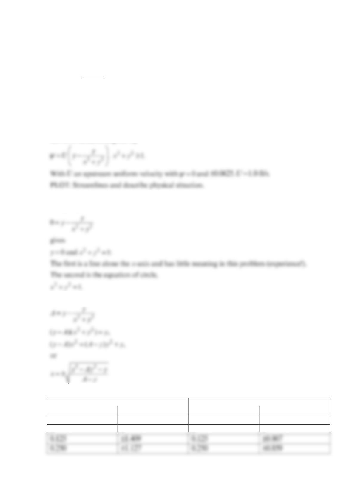
Streamlines are given in Cartesian coordinates by the equation.
22
y
Uy xy
ψ
=−
+
. 22
1xy+≥
.
Plot the streamlines for 0, 0.0625
ψ
=± , and describe the physical situation represented by
this equation. The parameter
U
is an upstream uniform velocity of
1.0 ft/
s
.
Solution 4.5
GIVEN: Streamline given by
SOLUTION:
For
0
ψ
=,
0
For ( 0.0625)A
ψ
==± ,
We now tabulate x versus
y
, for 0.062
5
A
= and 0.0625
A
=−
0.062
5
A
= 0.0625
A
=−
y
x
y
x
0 0 0 0
ψ
U
0
ψ
5
0.375 1.029
±
0.375 0.846
±
y
x
y
x
0 0 0 0
0.125
−
0.807
±
0.125
−
1.409
±
−
±
−
±
−
±
−
±
−
±
−
±
−
±
−
±
−
−
±
The values in the upper right section and lower left section of the table are not relevant
since they do not satisfy the condition that 22
1xy+≥
. The x,
y
values on the upper left
1.0
y
= +0.0625
ψ
±
±
±
Problem 4.6
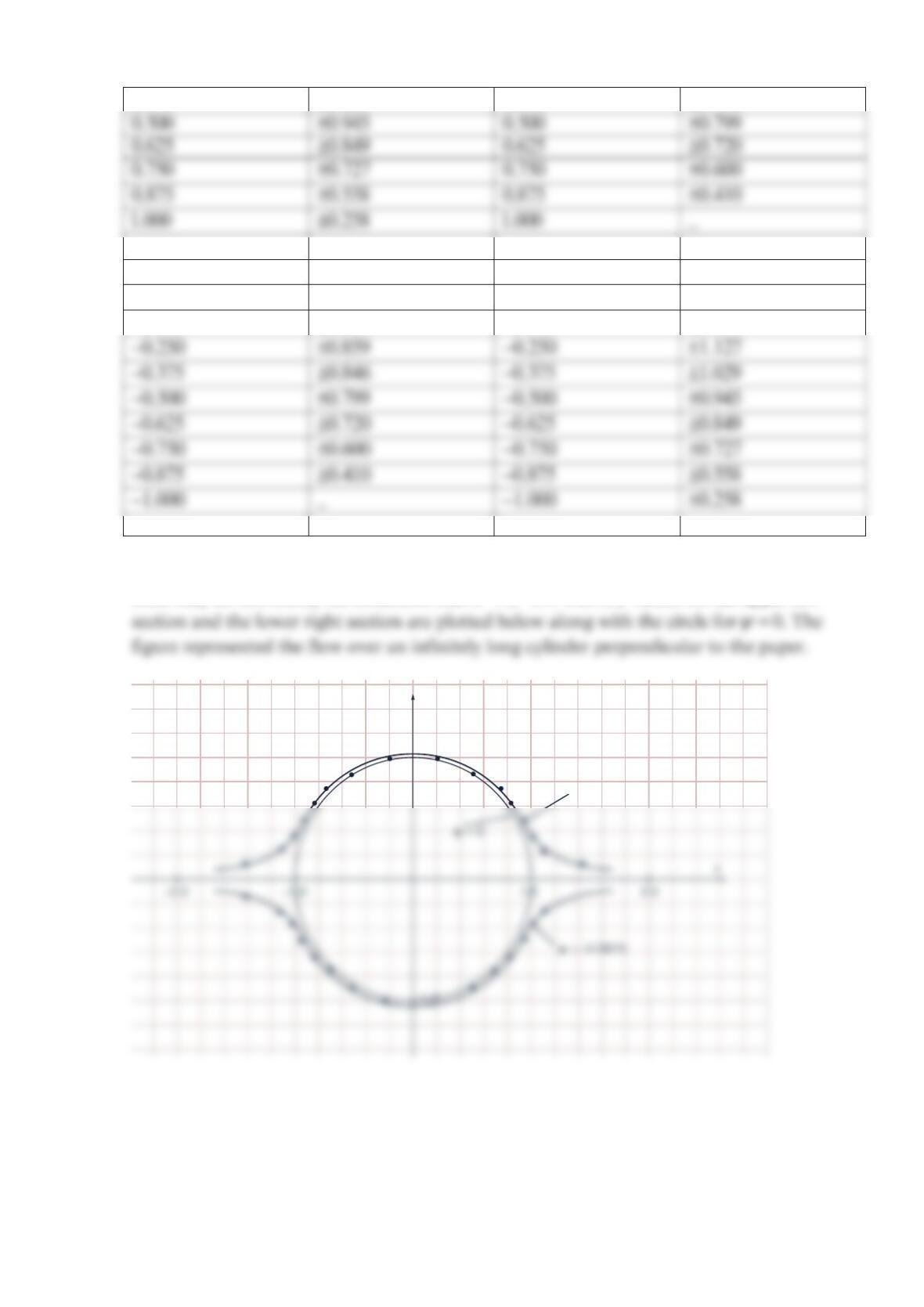
A flow can be visualized by plotting the velocity field as velocity vectors at representative
locations in the flow as shown in the figure below.
Consider the velocity field given in polar coordinates by 10
r
vr
=− , and 10
vr
θ
=. This flow
approximates a fluid swirling into a sink as shown in the figure below.
Plot the velocity field at locations given by 1, 2, and 3r= with 0 , 30 , 60 , and 90
θ
=
.
y
2ℓ
2
V0
2
V0
2
V0
V0
V0
V0
V0
/2
ℓ
−2ℓ
−ℓ
0
x
(
a
)
θ
V
u
(b)
v
(
c
)
y
V
= 0
x
r
v
vr
θ
θ
v
θ
V
0
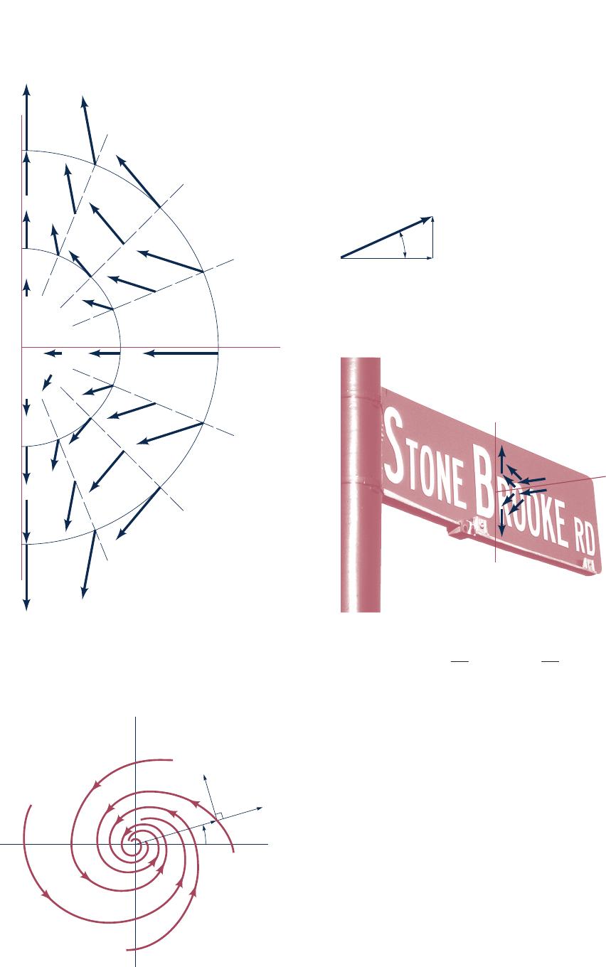
Solution 4.6
With 10
r
V
r
=− and 10
V
r
θ
= then
The angle
α
between the radial direction and the velocity vector
is given by
3
= 60
θ
Problem 4.7
A car accelerates from rest to a final constant velocity Vf and a police officer records the
following velocities at various locations x along the highway:
0x=.0mphV=
100ftx=34.8mphV=
200ftx=47.6 mphV=
300ftx=52.3mphV=
400ftx=54.0 mphV=
1000ftx=f
55.0 mphVV==
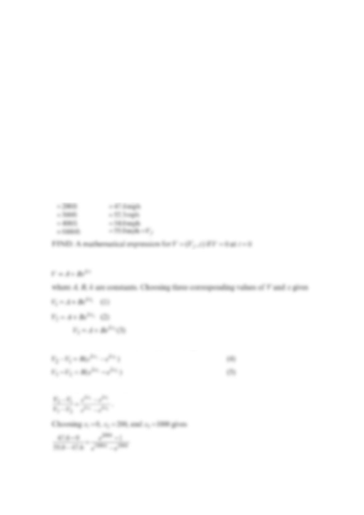
Find a mathematical Eulerian expression for the velocity V traveled by the car as a function
of the final velocity Vf of the car and x if 0t= at 0
V
=. [Hint: Try an exponential fit to the
data.]
Solution 4.7
GIVEN: Car accelerates from rest to Vf with
0x=0
V
=
100ft= 34.8mph=
SOLUTION: At suggested in the problem statement, we try an exponential form
Subtracting Eq. (1) from (2) and (2) from (3) gives
Dividing Eq. (4) by (5) gives
V
or
Then
Problem 4.8
The components of a velocity field are given by =+uxy
, =+
316vxy , and =0w.
Determine the location of any stagnation points (
0
V=) in the flow field.
Solution 4.8
=++=++ + =
22 2 2 3 2
()( 16)0Vuvw xy xy
Problem 4.9
A two-dimensional, unsteady velocity field is given by
=+5(1 )uxt
and =−+5(1 )vy t
,
where u is the x-velocity component and v the
y
-velocity component. Find ()xt and
()yt if =0
xx
and =0
y
y at =0t. Do the velocity components represent an Eulerian
description or a Lagrangian description?
Solution 4.9
GIVEN: Two-dimensional, unsteady flow with
SOLUTION: Start with
Separating variables and integrating gives
Problem 4.10
The velocity field of a flow is given by −
=
+
0
1
22
2
()
Vy
u
xy
and =
+
0
1
22
2
()
Vx
v
xy
, where 0
V is a
constant. Where in the flow field is the speed equal to 0
V? Determine the equation of the
streamlines and discuss the various characteristics of this flow.
Solution 4.10
=−
+
01
22
2
()
y
uV
xy
, =
+
01
22
2
()
x
vV
xy
so that
Problem 4.11
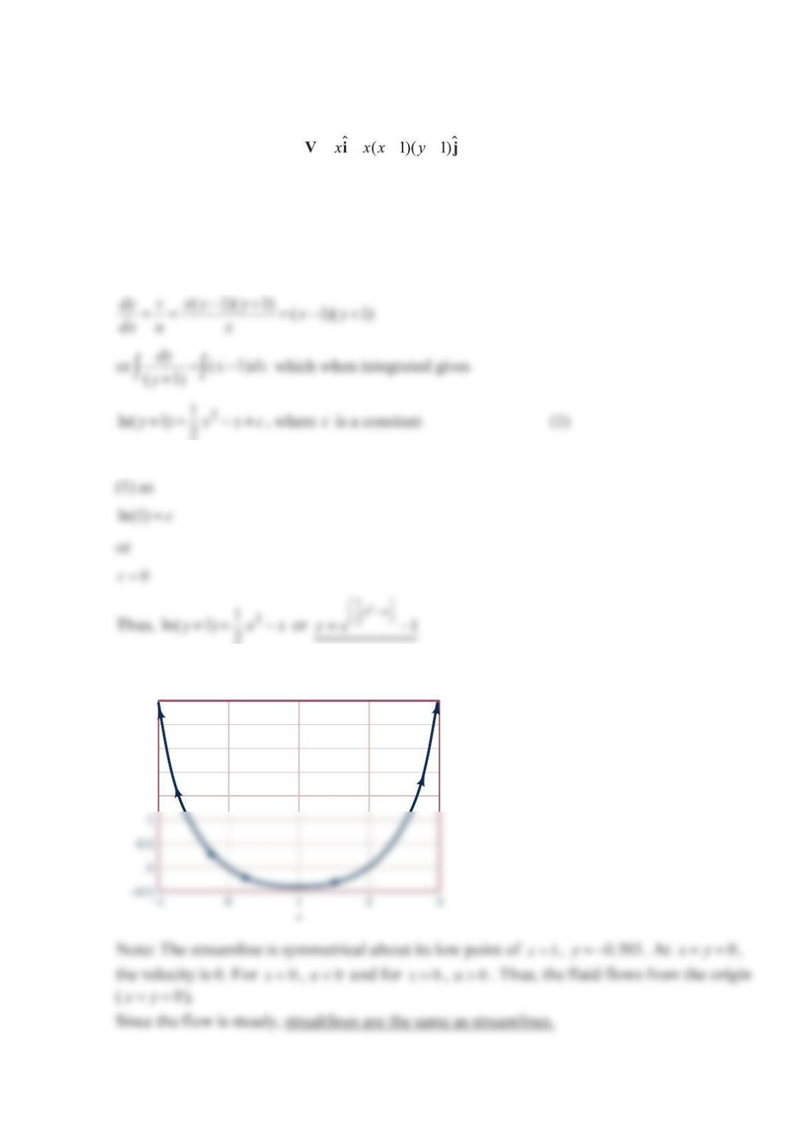
A velocity field is given by =+ − + , where u and v are in ft/s and x and
y
are in feet. Plot the streamline that passes through =0x and =0y. Compare this
streamline with the streakline through the origin.
Solution 4.11
=ux
, =−+(1)(1)vxx y where the streamlines are obtained from
For the streamline that passes through the origin ==0xy the value of c is found from Eq.
This streamline is plotted below
1.5
2
2.5
3
3.5
y
Problem 4.12
From time
0
t= to 5 hrt= radioactive steam is released from a nuclear power plant accident
located at 1 mil
e
x=− and 3 miles
y
=. The following wind conditions are expected:
10 5 mph=−V for 03 h
r
t<< , 15 +8 mph=V for 310 h
r
t<< , and 5mph=V for 10 h
r
t>.
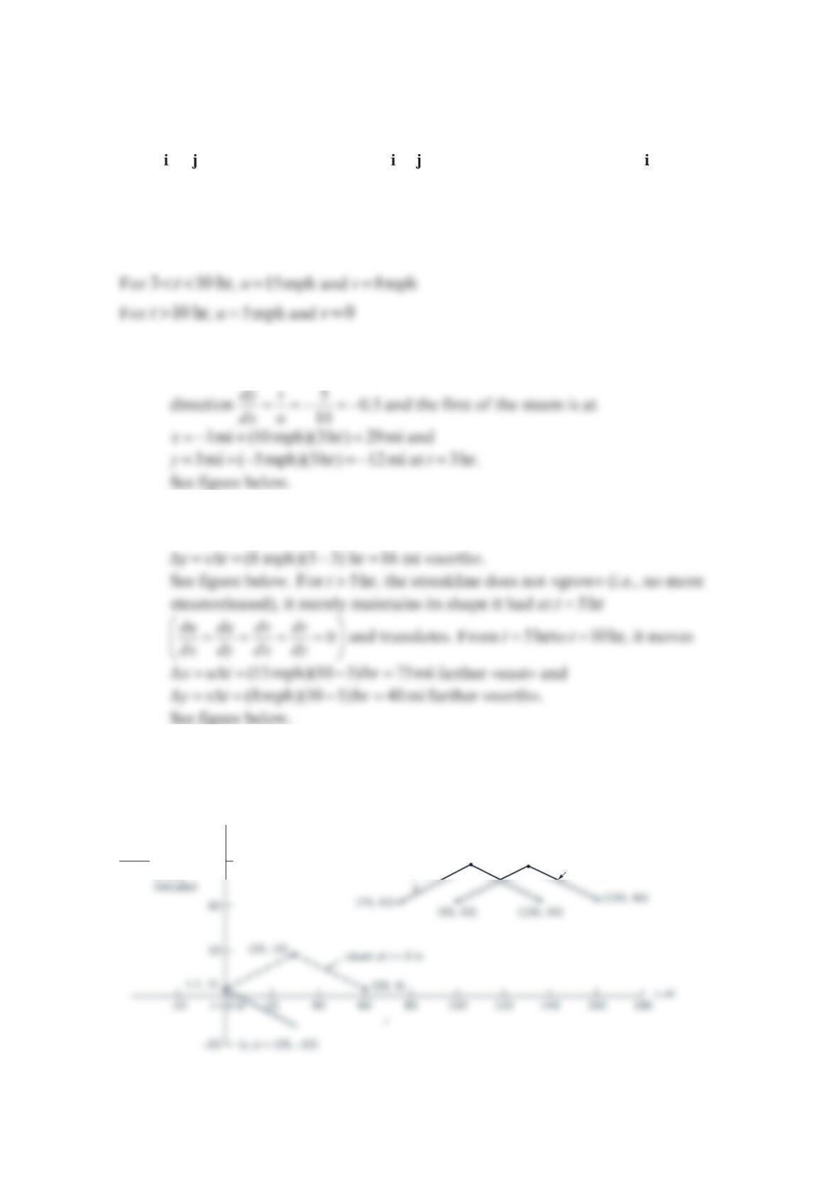
Draw to scale the expected streakline of the steam for 3, 10, and 15 hrt=.
Solution 4.12
For 03 h
r
t<< , 10 mphu= and 5mp
h
v=−
The streakline is the location (at time
t
) of steam released earlier.
a) At 3 hrt=, steam is still being released. From
0
t= to 3 hrt<, it has traveled in the
y
b) At 5hrt=, steam release stops. From 3hrt= to 5hrt=, the steams travels
(15 mph)(5 3) hr 30 mixut
Δ
=Δ= − = «east» and
Δ
Δ
c) For
1
015hrt<< , the steam moves (5 mph)(15 10) hr 25 mix
Δ
=−=
«east» and
0mi
y
vt
Δ
=Δ= «north».
The above is shown in the figure below.
y, mi
streakline
at time
t = 15 hr
t = 10 hr
(129, 59)(104, 59)
60
r
Problem 4.13
The x and
y
components of a velocity field are given by 2
uxy= and 2
vxy=− . Determine the
equation for the streamlines of this flow and compare it with those in the Example below. Is
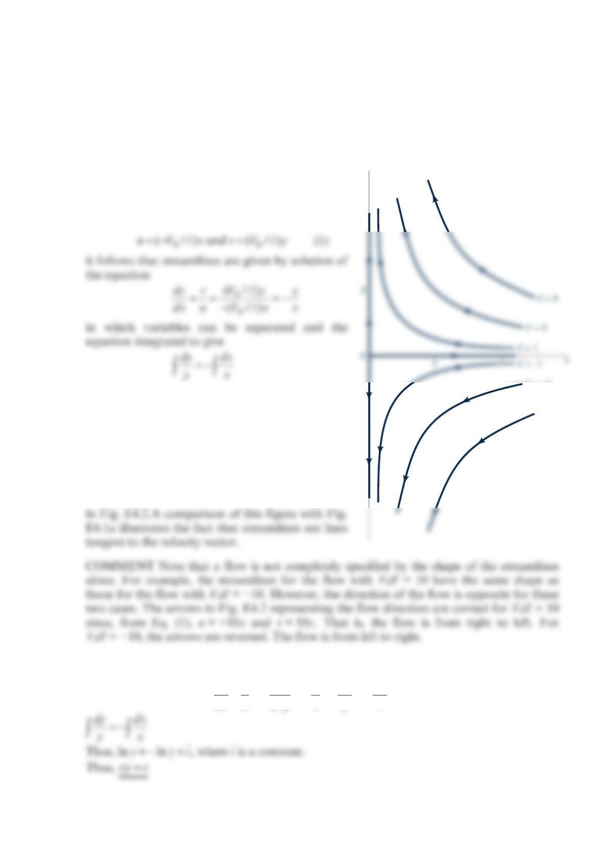
the flow in this problem the same as that in the Example below? Explain.
GIVEN: Consider the two-dimensional steady flow discussed in Example 4.1,
0ˆˆ
(/)( )Vxy
=−+Vij.
FIND: Determine the streamlines for this flow.
SOLUTION:
Since
or
ln ln constant
y
x=− +
Thus, along the streamline
=,xy C where C is a constant (Ans)
Using different values of the constant C, we can
plot various lines in the x−y plane—the
streamlines. The streamlines for x ≥ 0 are plotted
Solution 4.13
Streamlines are given by
2
2
dy v xy y
dx u x
y
==− =−
or dy dx
y
x
=− which can be integrated as:
y
4
–4
C
= –4
C
= –9
–2
Note: These streamlines are the same shape (same “flow pattern”) as in the Example given
Problem 4.14
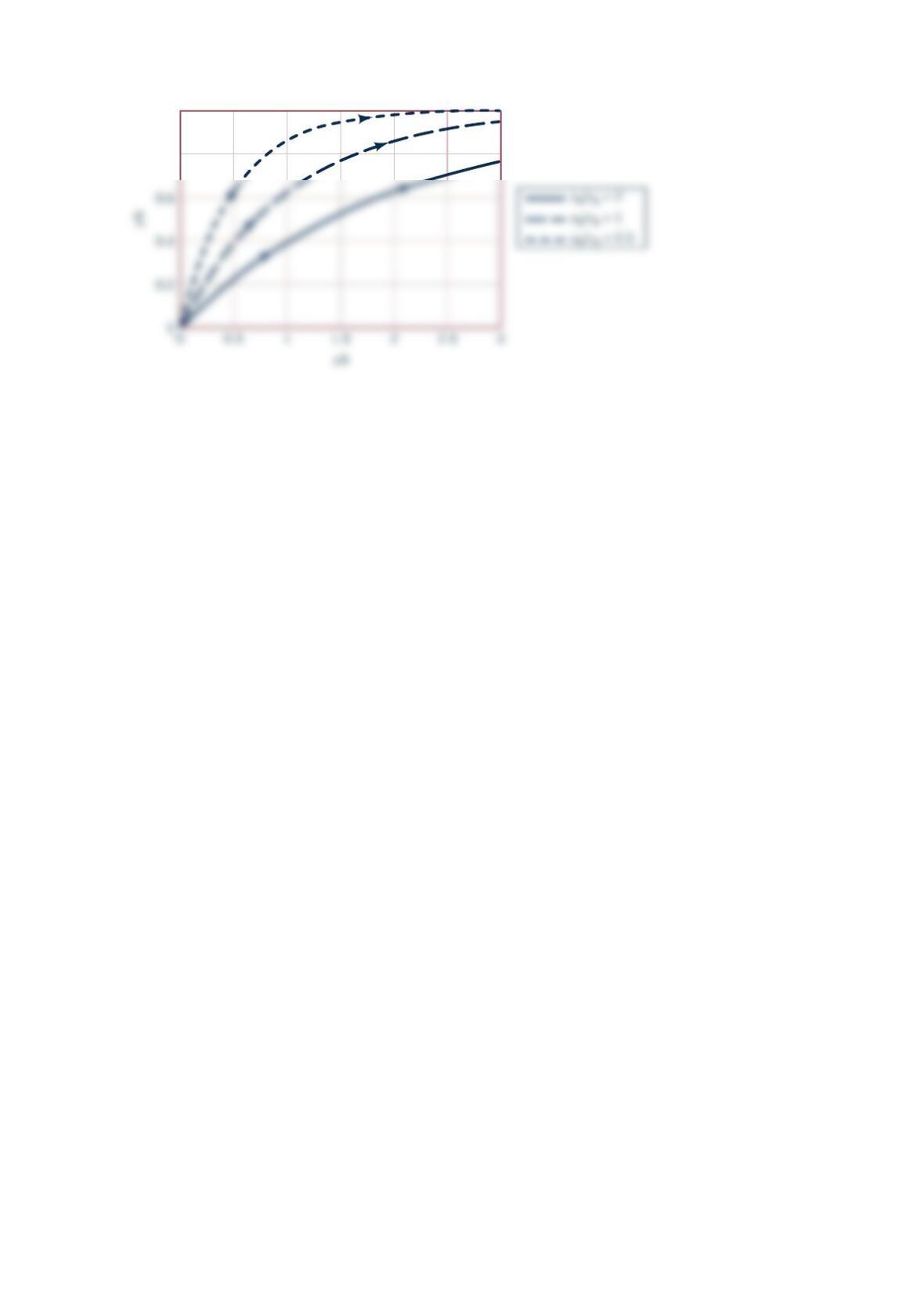
In addition to the customary horizontal velocity components of the air in the atmosphere
(the “wind”), there often are vertical air currents (thermals) caused by buoyant effects due
to uneven heating of the air as indicated in the figure below.
Assume that the velocity field in a certain region is approximated by =0
uu
, =−
0(1 )
y
vv h
for <<0yh
, and =0
uu
, =0v for >yh
. Plot the shape of the streamline that passes
through the origin for values of =
0
0
0.5, 1, and 2
u
v.
Solution 4.14
Thus, −−=
0
0
ln(1 ) v
y
hx
hu
u0
y
x
0
0.8
1
y/h vs x/h
Problem 4.15
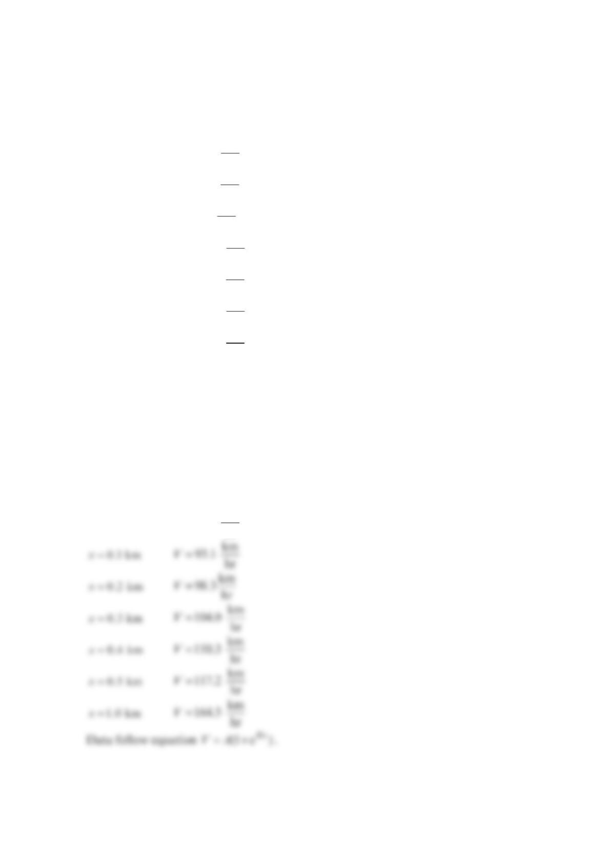
A test car is traveling along a level road at 88 km/hr. In order to study the acceleration
characteristics of a newly installed engine, the car accelerates at its maximum possible rate.
The test crew records the following velocities at various locations along the level road:
=0x=km
88.5 hr
V
=0.1 kmx=km
93.1 hr
V
=0.2 kmx=km
98.3 hr
V
=0.3 kmx=km
104.0 hr
V
=0.4 kmx=km
110.3 hr
V
=0.5 kmx=km
117.2 hr
V
=1.0 kmx=km
164.5 hr
V
A preliminary study shows that these data follow an equation of the form =+(1 e )
Bx
VA ,
where A and B are positive constants. Find A and B and a Lagrangian expression
=0
(,)VVVt
, where 0
V is the car velocity at time =0t when 0x=.
Solution 4.15
GIVEN: Car accelerates with
=0x=km
88.5 hr
V