Section 11.3: Frobenius Series Solutions 635
25. With exponent 1
1:
2
r 1
2
n
n
c
cn
26. With exponent 1
1:
2
r 2
10, n
n
c
cc
n
2
2
246 8
/2
1/2
1
0
() 1 !2
2 8 48 384
n
x
n
n
x
xxx x e
yx x x x
n
The differential equations in Problems 27–29 (after multiplication by x) and the one in Problem
31 are of the same form (1) above as those in Problems 21–24. However, now the exponents r1
and r2 = r1 1 do differ by an integer. Hence when we substitute the smaller exponent r = r2
into Equation (3), we find that c0 and c1 are both arbitrary, and that cn is given (for n 2)
by the recurrence relation in (4). Thus the smaller exponent r2 yields the general solution
01 12
() () ()
y
xcyxcyx in terms of the two linearly independent Frobenius series solutions
12
()and ().
y
xyx
27. Exponents 12
0and 1;rr with 2
9
1: (1)
n
n
c
rc
nn
636 Chapter 11: Power Series Methods
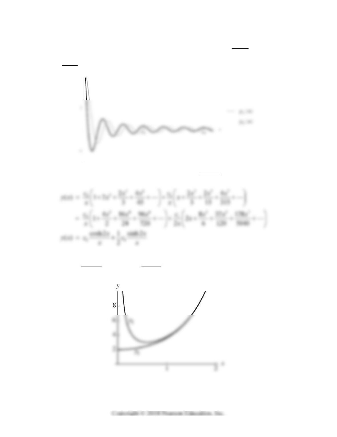
The figure below shows the graphs of the independent solutions 1
cos3
()
x
yx
x
and
2
sin 3
() .
x
yx
x
28. Exponents 12
0and 1;rr with 2
4
1: (1)
n
n
c
rc
nn
x
x
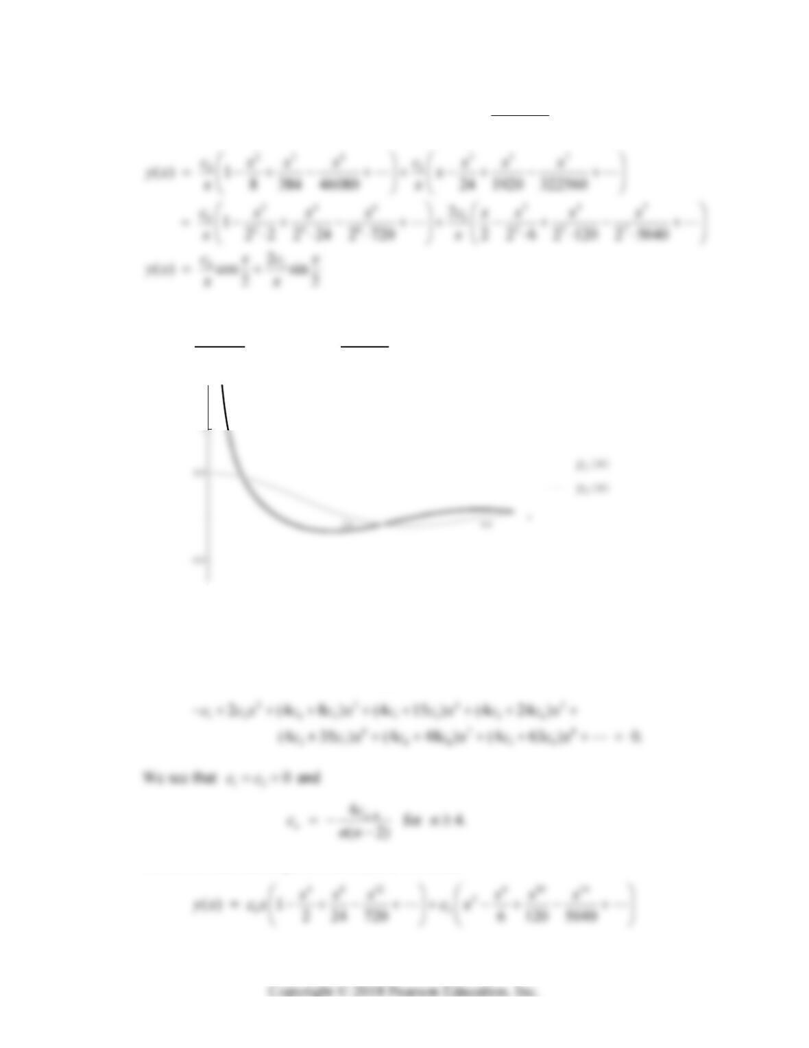
The figure below shows the graphs of the two independent solutions
12
cosh 2 sinh 2
() and () .
x
x
yx yx
xx
y
Section 11.3: Frobenius Series Solutions 637
29. Exponents 12
0and 1;rr with 2
1: 4( 1)
n
n
c
rcnn
The figure at the top of the next page shows the graphs of the independent solutions
12
cos / 2 sin / 2
() and () .
xx
yx yx
xx
30. The given differential equation 3
40xy y x y
has indicial equation
22(2)0,rrrr so its exponents are 12
2 and 0.rr Taking r = 0,
substitution of the power series
0
n
n
n
y
cx
gives
Hence the odd subscripts all vanish, and we obtain
y
638 Chapter 11: Power Series Methods
22
02
() cos sin .
y
xcxcx
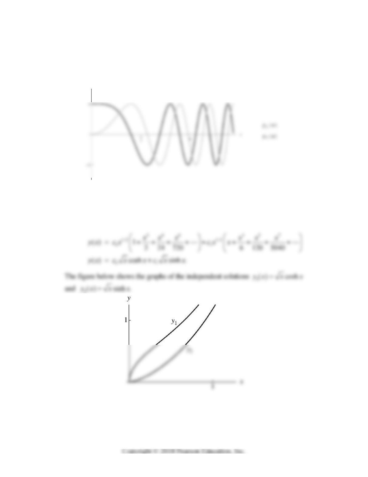
The figure below shows the graphs of the independent solutions 2
1() cosyx x
2
2
and ( ) sin .
y
xx
31. The given differential equation 22
44(34)0xy xy x y
has indicial equation
2
483(23)(21)0,rr r r so its exponents are 12
3/ 2 and 1/ 2.rr
With r = 3/2, the recurrence relation 2/( 1)
nn
ccnn
yields the general solution
32. The two indicial exponents are r1 = 1 and r2 = 1/2.
With r1 = 1: Substitution of n
n
yxcx in the differential equation yields
y
Section 11.3: Frobenius Series Solutions 639
With r2 = 1/2: We substitute 1/2 n
n
yx cx
and obtain the Frobenius solution
234
2
15155
() 1 .
2 8 48 384
xxxx
yx x
33. Exponents 12
1/2 and 1rr. With each exponent we find that c0 is arbitrary and
we can solve recursively for cn in terms of cn–1.
34. Exponents 12
1 and 1/ 2.rr With each exponent we find that c1 = 0 and we can
solve recursively for cn in terms of cn–2.
35. Substitution of rn
n
yx cx into the differential equation yields a result of the form
11
0() () 0,
rrr
rc x x x
640 Chapter 11: Power Series Methods
36. (a) Substitution of rn
n
yx cx into the differential equation 20x y Ay By
yields a result of the form
11
0() () 0,
rrr
Arc x x x
(c) Substitution of rn
n
yx cxinto the differential equation 32 0xy Axy By
yields a result of the form
37. Substitution of rn
n
yx cx into the differential equation 30xy xy y
yields a result of the form
Section 11.3: Frobenius Series Solutions 641
38. Exponents 12
1/2 and 1/2;rr with 2
1/2: (1)
n
n
c
rc
nn
39. Exponents 12
1and 1;rr with 2
1
1: 0, (2)
n
n
c
rcc
If c0 = 1/2, then
2
1
0
(1)
() () .
2!(1)2
n
n
n
xx
yx J x nn
Now, consider the smaller exponent r2 = –1. A Frobenius series with r = –1 is of the
form 1
0
n
n
n
y
xcx
with 00.c However, substitution of this series into Bessel’s
y
But this is the same as our series solution obtained above using the larger exponent
r = +1 (calling the arbitrary constant c2 rather than c0).
642 Chapter 11: Power Series Methods
SECTION 11.4
BESSEL FUNCTIONS
Of course Bessel’s equation is the most important special ordinary differential equation in
mathematics, and every student should be exposed at least to Bessel functions of the first kind.
1.
221
022 22
11
(1) (1)2
() 1 2(!) 2(!)
mm m m
xmm
mm
xmx
Jx D mm
2. (a) 21 21 21
222
nnn
(b)
1
2
1
2
221
1/ 2 2121
3
00
2
(1) 2 (1)
() !2 (2 1)!! 2
!( )2
m
mmm
mmm
mm
xx
Jx xmm
mm
3. (a) 232313434
33333
mmmm
m
Section 11.4: Bessel Functions 643
(b)
21/3 1/3 2
1/3
00
(1) (/2) (1)3
() !( 2/3) 2 (2/3) !238 (3 1)
m
mmmm
mm
xx x
Jx mm m m
4. With p = 1/2 in Equation (26) in the text we have
5. Starting with p = 3 in Equation (26) we get
8. When we carry out the differentiations indicated in Equations (22) and (23) in the text,
we get
9. (p + m + 1) = (p + m)(p + m 1)(p + 2)(p + 1)(p + 1), so
10. Substitution of the power series of Problem 9 yields
644 Chapter 11: Power Series Methods
D = (1/21/2)(1/2). Hence
x
11. 2
00
() ()
x
Jxdx xxJxdx
x
x
12. 32
00
() ()
x
J x dx x xJ x dx
x
13. 43
00
() ()
x
Jxdx xxJxdx
x
x
14. 1100
() () () ()
x
Jxdx xJxdx xJx JxdxC
x
x
Section 11.4: Bessel Functions 645
16. 33
11
() ()
x
Jxdx xJxdx
x
x
17. 44
11
() ()
x
Jxdx xJxdx
x
x
18. With p = 1, Eq. (23) in the text gives 11
21
() () .
x
Jxdx xJx C
Hence
Problems 19–30 are routine applications of the theorem in this section. In each case it is
necessary only to identify the coefficients A, B, C and the exponent q in the differential
equation
2()0.
q
xy Axy B Cx y
(1)
Then we can calculate the values
646 Chapter 11: Power Series Methods
specified in Theorem 1 on solutions in terms of Bessel functions. This is a “template procedure”
that we illustrate only in a couple of problems.
19. We hav e 1, 1, 1, 2ABCq so
20. y(x) = x1[c1J1(x) + c2Y1(x)]
23. To match the given equation with Eq. (1) above, we first divide through by the leading
coefficient 16 to obtain the equation
24. y(x) = x1/4 [c1J0(2x3/2) + c2Y0(2x3/2)]
25. y(x) = x1[c1J0(x) + c2Y0(x)]
Section 11.4: Bessel Functions 647
30. y(x) = x1/2 [c1J1/5(4x5/2/5) + c2J1/5(4x5/2/5)]
31. We want to solve the equation xy” + 2y’ + xy = 0. If we rewrite it as
ii
33. The substitution
2
2
()
,
uuu
yy
uuu
immediately transforms y’ = x2 + y2 to u” + x2u = 0. The equivalent equation
x2u” + x4u = 0
648 Chapter 11: Power Series Methods
1/2 2 1/4 1/ 4 3/ 2 2
1/ 4 1/ 4 3/ 4
(/2) 2 () (/2).
dddz
xJ x zJ z xJ x
dx dz dx
34. Substitution of the series expressions for the Bessel functions in the formula for y(x) in
Problem 33 yields
where each pair of parentheses encloses a power series in x with constant term 1, and
A = 23/4 /(7/4) B = 23/4 /(1/4)
C = 21/4 /(5/4) D = 21/4 /(3/4).
Multiplication of numerator and denominator by x1/2 and a bit of simplification gives
(a) If y(0) = 0 then (*) gives c = 0 in the general solution formula of Problem 33.
(b) If y(0) = 1 then (*) gives c = (1/4)/2(3/4). More generally, (*) yields the
formula
APPENDIX A
EXISTENCE AND UNIQUENESS OF SOLUTIONS
In Problems 1–12 we apply the iterative formula
starting with y0(x) = b.
1. y0(x) = 3
y1(x) = 3 + 3x
2. y0(x) = 4
y1(x) = 4 – 8x
3. y0(x) = 1
y1(x) = 1 – x2
650 Appendix A
4. y0(x) = 2
y1(x) = 2 + 2x3
5. y0(x) = 0
y1(x) = 2x
6. y0(x) = 0
y1(x) = (1/2)x2
7. y0(x) = 0
y1(x) = x2
Existence and Uniqueness of Solutions 651
8. y0(x) = 0
y1(x) = 2x4
9. y0(x) = 1
y1(x) = (1 + x) + x2/2
10. y0(x) = 0
y1(x) = x + (1/2)x2 + (1/6)x3 + (1/24)x4 + = ex – 1
11. y0(x) = 1
y1(x) = 1 + x
12. y0(x) = 1
y1(x) = 1 + (1/2)x
652 Appendix A
13. 0
0
() 1
() 1
xt
yt
14.
0
11
1
() 01 1
!
n
n
n
tt
n
x
16. y0(x) = 0
y1(x) = (1/3)x3
y2(x) = (1/3)x3 + (1/63)x7
Existence and Uniqueness of Solutions 653
2
1
3/4 2
2
1
1/4 2
() Jx
yx x Jx
so the exact value at x = 1 is