PROBLEM 4.71 (Cont.)
COMMENTS: (1) The IHT Workspace for the 5×5 coarse node analysis with results follows.
// Finite–difference equations – energy balances
// First row – treating as interior nodes considering symmetry
T1 = 0.25 * ( Tc + T2 + T4 + T2 )
T2 = 0.25 * ( Tc + T3 + T5 + T1 )
T3 = 0.25 * ( Tc + T2 + T6 + T2 )
/* Second row – Node 4 treat as interior node; for others, use Tools: Finite–Difference Equations,
/* Third row – Node 7 treat as interior node; for others, use Tools: Finite–Difference Equations,
Two–Dimensional, Steady–State; be sure to delimit replicated q”a = 0 equations. */
T7 = 0.25 * (T4 + T8 + T9 + T8)
/* Node 8: plane surface node, e–orientation; w, n, s labeled 7, 5, 10. */
0.0 = fd_2d_psur_e(T8,T7,T5,T10,k,qdot,deltax,deltay,Tinf,h,q’‘a)
//q”a = 0 // Applied heat flux, W/m^2; zero flux shown
/* Fourth row – Node 9 treat as interior node; for others, use Tools: Finite–Difference Equations,
// Assigned variables
// For the FDE functions,
qdot = 0 // Volumetric generation, W/m^3
/* Heat rate per unit length, for two symmetrical elements about one microchannel, */
q’cv= 2 * (q’5 + q’6 + q’8 + q’10)
/* Thermal resistance between chip and fluid, per unit channel length, */
R’tcf = (Tc – Tinf) / q’cv // Thermal resistance, m.K/W
// Total power for a chip of 10mm x 10mm, Pchip (W),
q”c = q’cv / (wf + ws) // Heat flux on chip surface, W/m^2
Pchip = Achip * q”c // Power, W
Achip = 0.01 * 0.01 // Chip area, m^2
PROBLEM 4.72
KNOWN: Long rectangular bar having one boundary exposed to a convection process (T∞, h) while the
other boundaries are maintained at a constant temperature (Ts).
FIND: (a) Using a grid spacing of 30 mm and the Gauss-Seidel method, determine the nodal
temperatures and the heat rate per unit length into the bar from the fluid, (b) Effect of grid spacing and
convection coefficient on the temperature field.
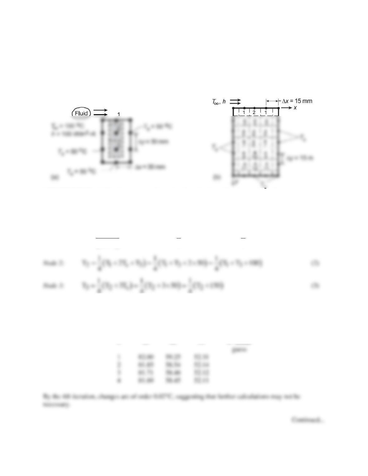
SCHEMATIC:
ASSUMPTIONS: (1) Steady-state, two-dimensional conduction, (2) Constant properties.
ANALYSIS: (a) With the grid spacing ∆x = ∆y = 30 mm, three nodes are created. Using the finite-
difference equations as shown in Table 4.2, but written in the form required of the Gauss-Seidel method
(see Appendix D), and with Bi = h∆x/k = 100 W/m2⋅K × 0.030 m/1 W/m⋅K = 3, we obtain:
Node 1:
( ) ( ) ( ) ( )
1 2s 2 2
1 11
T T T BiT T 50 3 100 T 350
Bi 2 5 5
∞
= + + = + +× = +
+
(1)
Denoting each nodal temperature with a superscript to indicate iteration step, e.g.
k
1
T
, calculate values
as shown below.
k
T1
T2
T3 (°C)
0
85
60
55
← initial
PROBLEM 4.72 (Cont.)
In finite–difference form, the heat rate from the fluid to the bar is
( )( ) ( ) ( )( )
conv s 1 s
q hx2TThxTThx2TT
∞∞ ∞
′=∆−+∆−+∆−
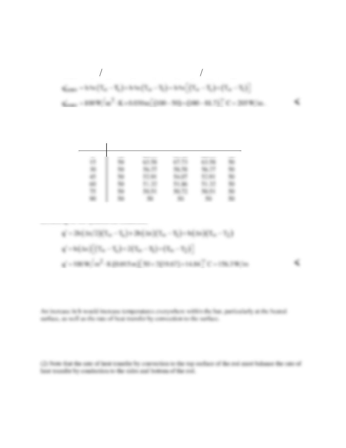
(b) Using the Finite-Difference Equations option from the Tools portion of the IHT menu, the following
two-dimensional temperature field was computed for the grid shown in schematic (b), where x and y are
in mm and the temperatures are in °C.
y\x
0
15
30
45
60
0
50
50
50
50
50
50
50
50
50
50
The improved prediction of the temperature field has a significant influence on the heat rate, where,
accounting for the symmetrical conditions,
Additional improvements in accuracy could be obtained by reducing the grid spacing to 5 mm, although
the requisite number of finite-difference equations would increase from 12 to 108, significantly
increasing problem set-up time.
COMMENTS: (1) Using the matrix-inversion method, the exact solution to the system of equations (1,
2, 3) of part (a) is T1 = 81.70°C, T2 = 58.44°C, and T3 = 52.12°C. The fact that only 4 iterations were
required to obtain agreement within 0.01°C is due to the close initial guesses.
PROBLEM 4.73
KNOWN: Thickness of a porous plane wall and its surface temperatures. Expression for effective
thermal conductivity including effect of radiation. Grid spacing, ∆x.
FIND: Nodal temperatures and wall heat flux. Importance of radiation.
SCHEMATIC:
x
ASSUMPTIONS: (1) Steady–state conditions, one-dimensional conditions, (2) No internal heat
generation.
PROPERTIES: Given: keff,r+c = 4.0 W/m⋅K +
s
T3
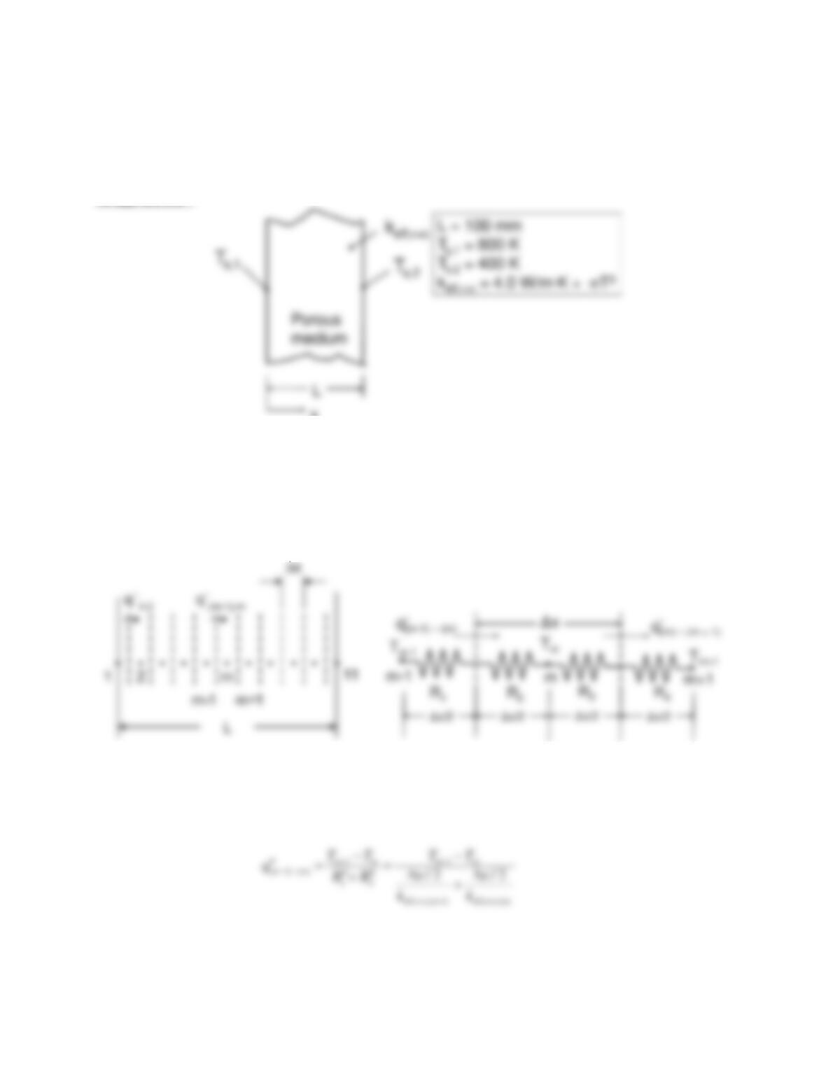
ANALYSIS: The discretized solution domain (left) and heat fluxes and resistances for a general interior
node (right) are shown below.
Recognizing that the effective conductivity is a function of temperature, and temperature is only
calculated at the nodes, the thermal resistance between nodes m-1 and m is evaluated in two pieces
(shown as R1 and R2 above), using the temperatures at the nodes. Thus the heat flux from node m-1 to m is
given by
Continued…
PROBLEM 4.73 (Cont.)
Similarly,
We may write similar expressions for nodes 2 through 10, noting that the heat flux must be constant
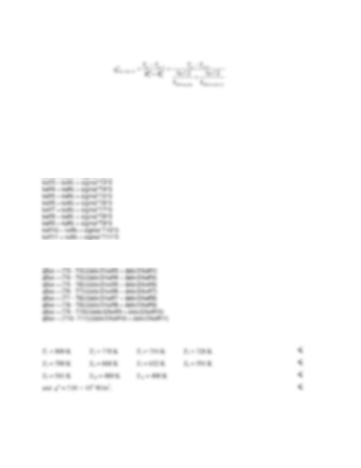
through the entire wall. At nodes 1 and 11, the temperatures are specified. The IHT code is:
sigma = 5.67e-8
T1 = 800
T11 = 400
keffc = 4
delx = 0.01
//Evaluate effective thermal conductivity for radiation and conduction at each node.
keff1 = keffc + sigma*T1^3
keff2 = keffc + sigma*T2^3
//Write an expression for the heat flux between each pair of nodes, recognizing that heat flux is constant.
qflux = (T1 – T2)/(delx/2/keff1 + delx/2/keff2)
qflux = (T2 – T3)/(delx/2/keff2 + delx/2/keff3)
The solution to the finite difference equations is:
Continued…
PROBLEM 4.73 (Cont.)
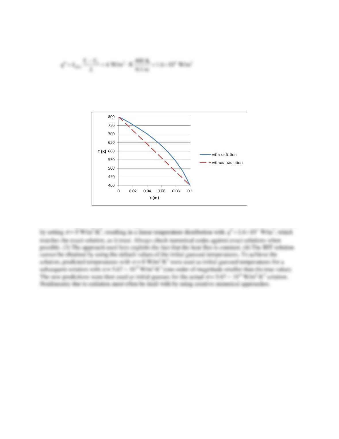
Neglecting the radiation contribution to the heat flux yields
Therefore radiation significantly increases the heat transfer rate. <
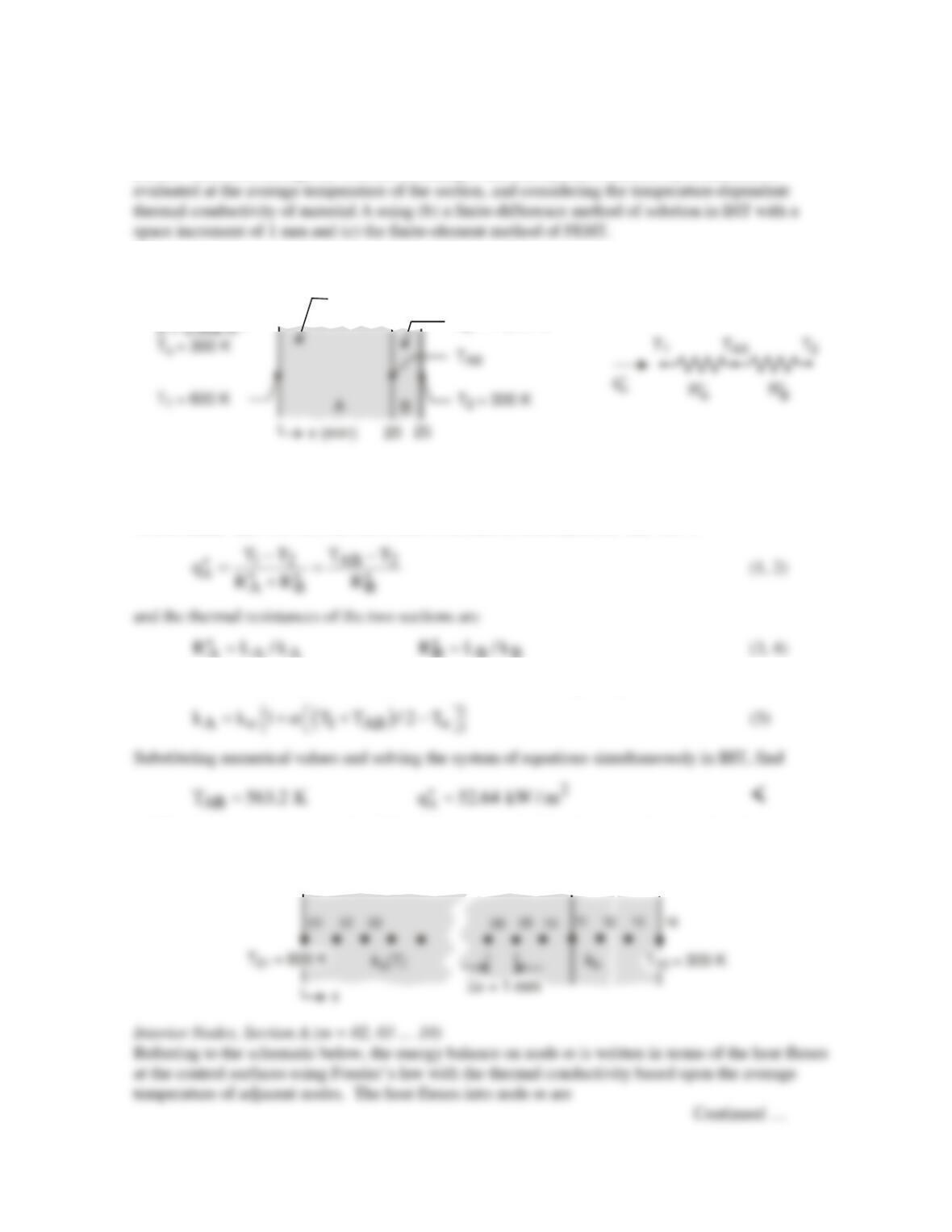
COMMENTS: (1) The temperatures calculated with and without radiation are shown below.
It can be seen that small temperature gradients are associated with large effective thermal conductivities
that occur at high temperature due to significant radiation. (2) The numerical (IHT) code can be modified
PROBLEM 4.74
KNOWN: Plane composite wall with exposed surfaces maintained at fixed temperatures. Material A
has temperature–dependent thermal conductivity.
FIND: Heat flux through the wall (a) assuming a uniform thermal conductivity in material A
SCHEMATIC:
kb = 1 W/m-K
kk T
a o o
= [1 + (T- )]
a
k
o
= 4.4 W/m-K
-1
ASSUMPTIONS: (1) Steady-state, one-dimensional conduction, (2) No thermal contact resistance
between the materials, and (3) No internal generation.
ANALYSIS: (a) From the thermal circuit in the above schematic, the heat flux is
A AA B BB
The thermal conductivity of material A is evaluated at the average temperature of the section
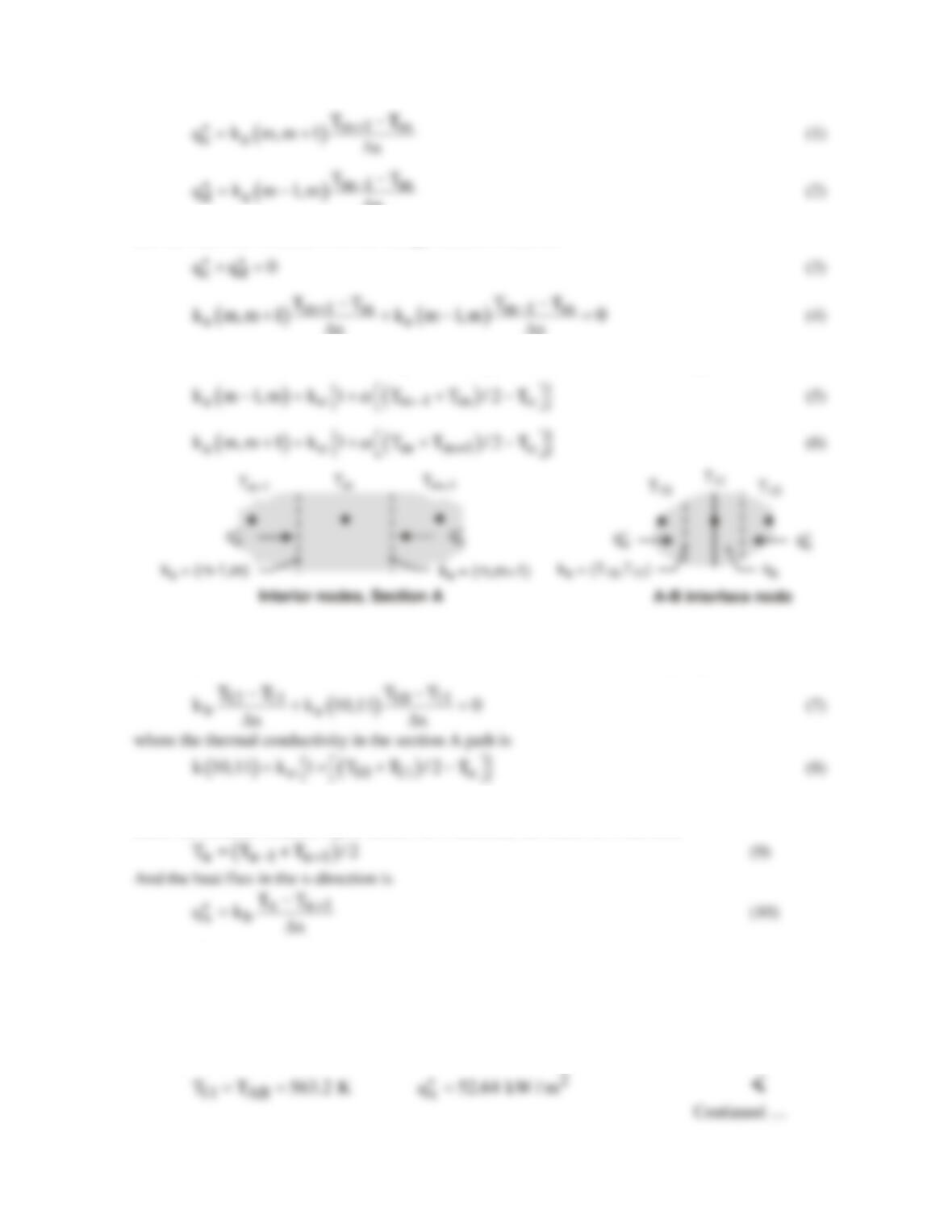
(b) The nodal arrangement for the finite-difference method of solution is shown in the schematic
below. FDEs must be written for the internal nodes (02 – 10, 12 – 15) and the A-B interface node
(11) considering in section A, the temperature-dependent thermal conductivity.
PROBLEM 4.74 (Cont.)
and the FDEs are obtained from the energy balance written as
xx
∆∆
where the thermal conductivities averaged over the path between the nodes are expressed as
A-B Interface Node 11
Referring to the above schematic, the energy balance on the interface node,
cd
q q 0,
′′ ′′
+=
has the form
Interior Nodes, Section B (n = 12 …15)
Since the thermal conductivity in Section B is uniform, the FDEs have the form
Finite-Difference Method of Solution
The foregoing FDE equations for section A nodes (m = 02 to 10), the AB interface node and their
respective expressions for the thermal conductivity, k (m, m +1), and for section B nodes are entered
into the IHT workspace and solved for the temperature distribution. The heat flux can be evaluated
using Eq. (2) or (10). A portion of the IHT code is contained in the Comments, and the results of the
analysis are tabulated below.
PROBLEM 4.74 (Cont.)
(c) The finite–element method of FEHT can be used readily to obtain the heat flux considering the
temperature–dependent thermal conductivity of section A. Draw the composite wall outline with
COMMENTS: (1) The results from the three methods of analysis compare very well. Because the
thermal conductivity in section A is linear, and moderately dependent on temperature, the simplest
method of using an overall section average, part (a), is recommended. This same method is
recommended when using tabular data for temperature-dependent properties.
(2) For the finite-difference method of solution, part (b), the heat flux was evaluated at several nodes
(3) To illustrate the use of IHT in solving the finite–difference method of solution, lines of code for
representative nodes are shown below.
// FDEs – Section A
k01_02 * (T01–T02)/deltax + k02_03 * (T03–T02)/deltax = 0
PROBLEM 4S.1
KNOWN: Long furnace of refractory brick with prescribed surface temperatures and material
thermal conductivity.
FIND: Shape factor and heat transfer rate per unit length using the flux plot method
SCHEMATIC:
ASSUMPTIONS: (1) Furnace length normal to page,
,
>> cross-sectional dimensions, (2) Two-
dimensional, steady-state conduction, (3) Constant properties.
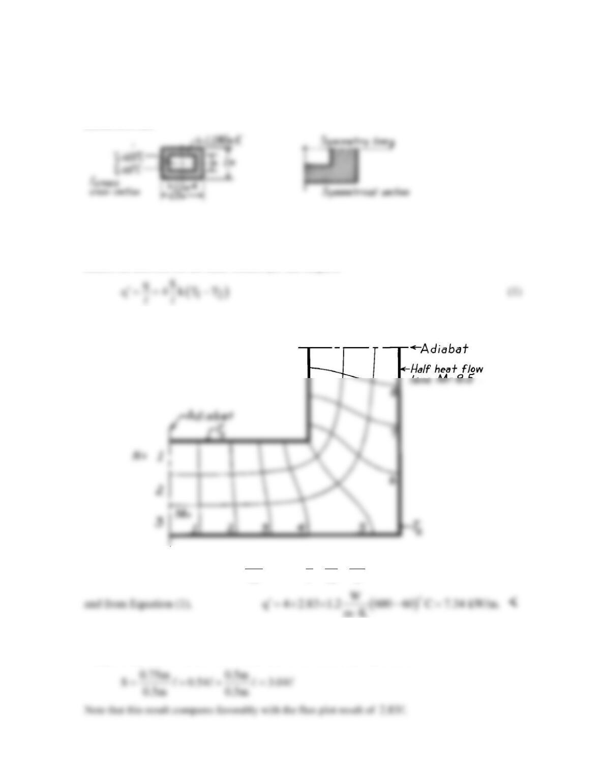
ANALYSIS: Considering the cross–section, the cross–hatched area represents a symmetrical element.
Hence, the heat rate for the entire furnace per unit length is
where S is the shape factor for the symmetrical section. Selecting three temperature increments ( N =
3), construct the flux plot shown below.
From Equation 4S.7,
M S M 8.5
S or 2.83
N N3
= = = =
<
q 4 2.83 1.2 600 60 C 7.34 kW/m.
COMMENTS: The shape factor can also be estimated from the relations of Table 4.1. The
symmetrical section consists of two plane walls (horizontal and vertical) with an adjoining edge.
Using the appropriate relations, the numerical values are, in the same order,
PROBLEM 4S.2
KNOWN: Hot pipe embedded eccentrically in a circular system having a prescribed thermal
conductivity.
FIND: The shape factor and heat transfer per unit length for the prescribed surface
temperatures.
SCHEMATIC:
ASSUMPTIONS: (1) Two-dimensional conduction, (2) Steady-state conditions, (3) Length
>> diametrical dimensions.
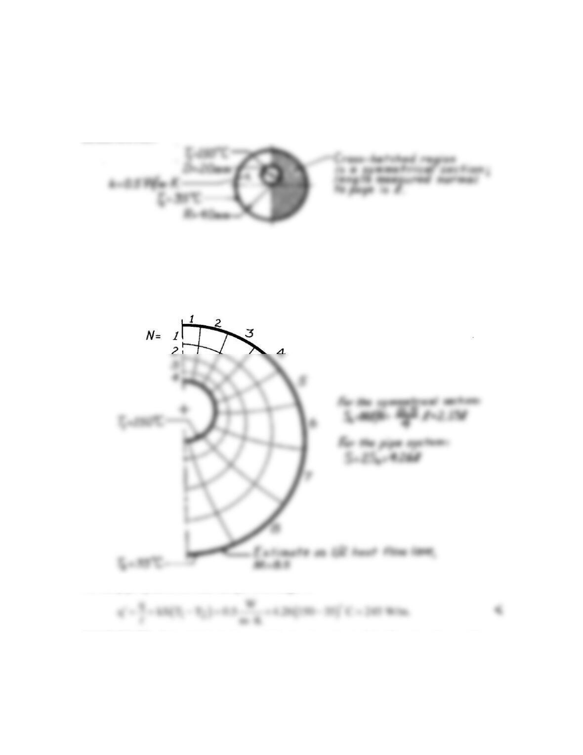
ANALYSIS: Considering the cross-sectional view of the pipe system, the symmetrical
section shown above is readily identified. Selecting four temperature increments (N = 4),
construct the flux plot shown below.
For the pipe system, the heat rate per unit length is
COMMENTS: Note that in the lower, right-hand quadrant of the flux plot, the curvilinear
squares are irregular. Further work is required to obtain an improved plot and, hence, obtain a
more accurate estimate of the shape factor.
PROBLEM 4S.3
KNOWN: Structural member with known thermal conductivity subjected to a temperature difference.
FIND: (a) Temperature at a prescribed point P, (b) Heat transfer per unit length of the strut, (c) Sketch
the 25, 50 and 75°C isotherms, and (d) Same analysis on the shape but with adiabatic–isothermal
boundary conditions reversed.
ASSUMPTIONS: (1) Two–dimensional conduction, (2) Steady-state conditions, (3) Constant
properties.
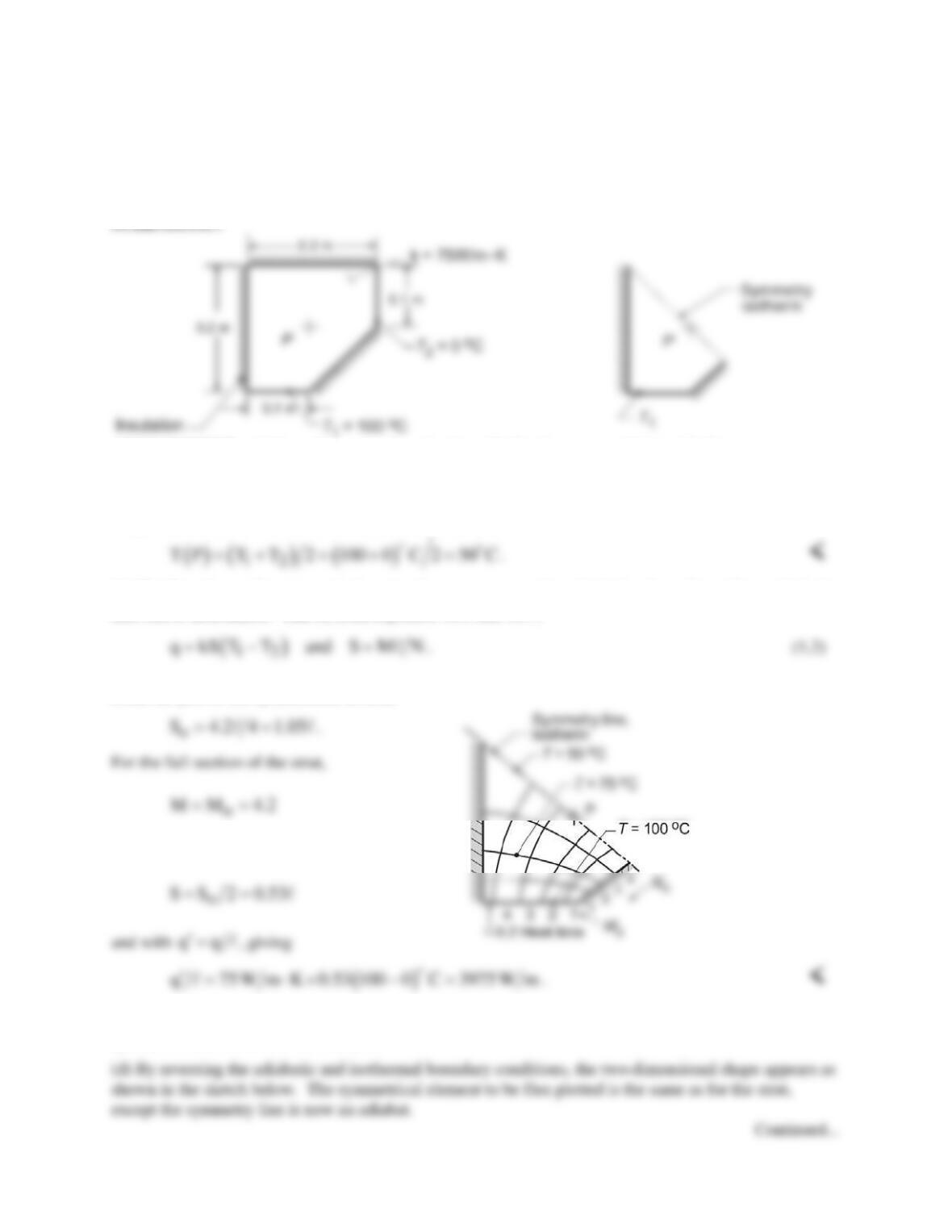
ANALYSIS: (a) When constructing the flux plot, note that the line of symmetry which passes through
the point P is an isotherm as shown above. It follows that
(b) The flux plot on the symmetrical section is now constructed to obtain the shape factor from which the
heat rate is determined. That is, from Equation 4S.6 and 4S.7,
From the plot of the symmetrical section,
but N = 2No = 8. Hence,
(c) The isotherms for T = 50, 75 and 100°C are shown on the flux plot. The T = 25°C isotherm is
symmetric with the T = 75°C isotherm.
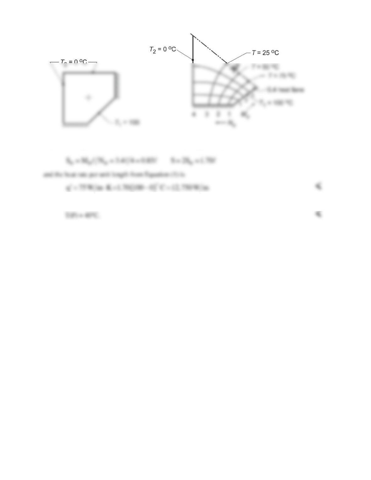
PROBLEM 4S.3 (Cont.)
From the flux plot, find Mo = 3.4 and No = 4, and from Equation (2)
From the flux plot, estimate that
COMMENTS: (1) By inspection of the shapes for parts (a) and (b), it is obvious that the heat rate for
the latter will be greater. The calculations show the heat rate is greater by more than a factor of three.
(2) By comparing the flux plots for the two configurations, and corresponding roles of the adiabats and
isotherms, would you expect the shape factor for parts (a) to be the reciprocal of part (b)?
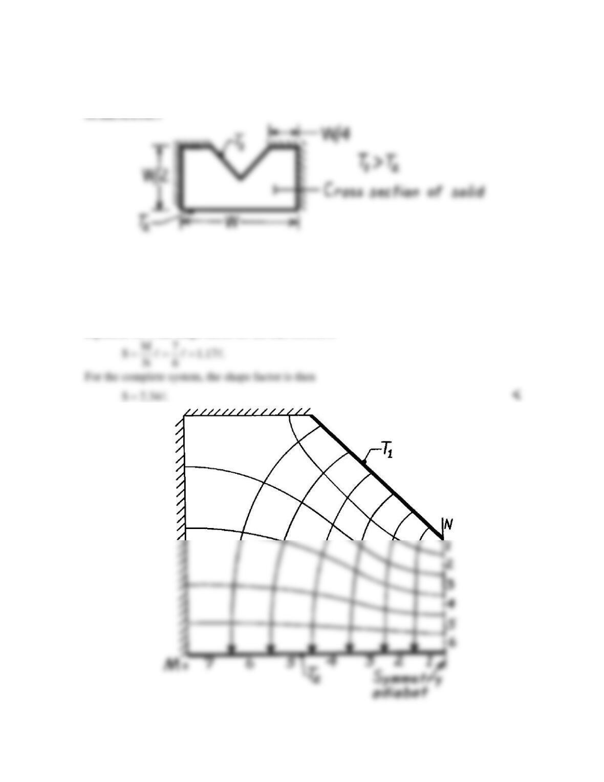
PROBLEM 4S.4
KNOWN: Relative dimensions and surface thermal conditions of a V-grooved channel.
FIND: Flux plot and shape factor.
ASSUMPTIONS: (1) Two-dimensional conduction, (2) Steady-state conditions, (3)
Constant properties.
ANALYSIS: With symmetry about the midplane, only one-half of the object need be
considered as shown below.
Choosing 6 temperature increments (N = 6), it follows from the plot that M ≈ 7. Hence from
Equation 4S.7, the shape factor for the half section is
PROBLEM 4S.5
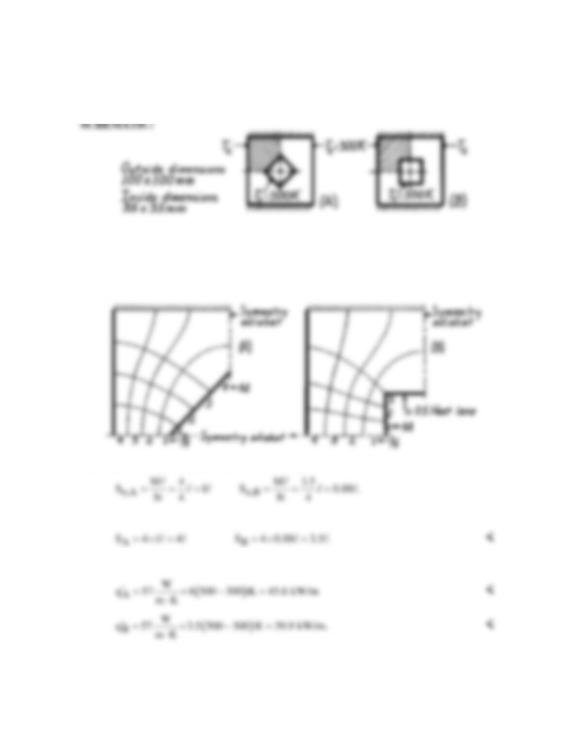
KNOWN: Long conduit of inner circular cross section and outer surfaces of square cross section.
FIND: Shape factor and heat rate for the two applications when outer surfaces are insulated or
maintained at a uniform temperature.
ASSUMPTIONS: (1) Two–dimensional, steady-state conduction, (2) Constant properties and (3)
Conduit is very long.
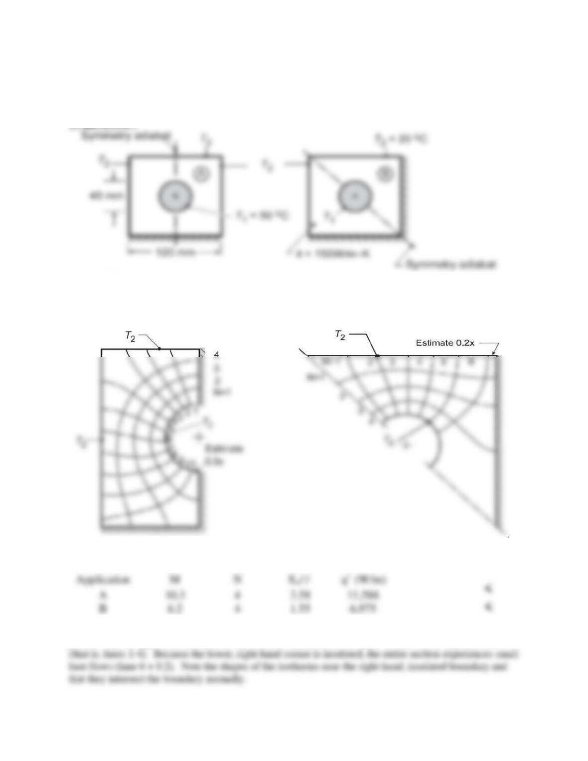
ANALYSIS: The adiabatic symmetry lines for each of the applications is shown above. Using the flux
plot methodology and selecting four temperature increments (N = 4), the flux plots are as shown below.
For the symmetrical sections, S = 2So, where So = M
/N and the heat rate for each application is q =
2(So/
)k(T1 – T2).
COMMENTS: (1) For application A, most of the heat lanes leave the inner surface (T1) on the upper
portion. (2) For application B, most of the heat flow lanes leave the inner surface on the upper portion
PROBLEM 4S.6
KNOWN: Shape and surface conditions of a support column.
FIND: (a) Heat transfer rate per unit length. (b) Height of a rectangular bar of equivalent
thermal resistance.
ASSUMPTIONS: (1)Steady-state conditions, (2) Negligible three-dimensional conduction
effects, (3) Constant properties, (4) Adiabatic sides.
PROPERTIES: Table A-1, Steel, AISI 1010 (323K): k = 62.7 W/m⋅K.
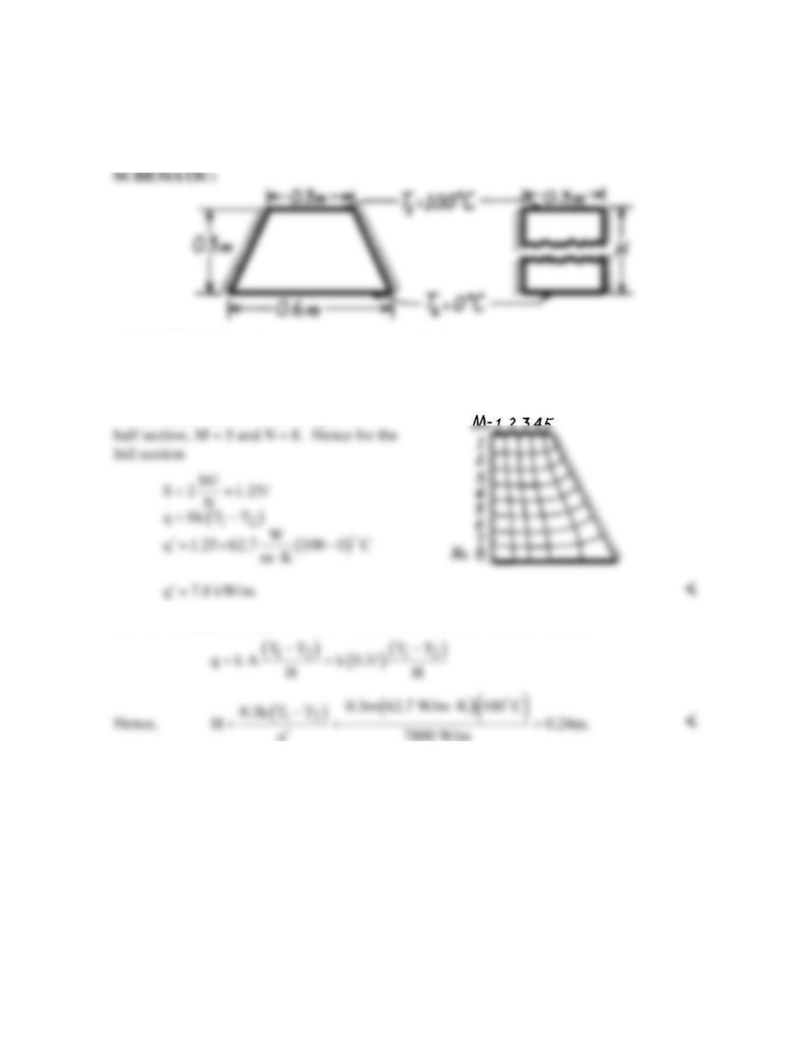
ANALYSIS: (a) From the flux plot for the
(b) The rectangular bar provides for one-dimensional heat transfer. Hence,
COMMENTS: The fact that H < 0.3m is consistent with the requirement that the thermal
resistance of the trapezoidal column must be less than that of a rectangular bar of the same
height and top width (because the width of the trapezoidal column increases with increasing
distance, x, from the top). Hence, if the rectangular bar is to be of equivalent resistance, it
must be of smaller height.
PROBLEM 4S.7
KNOWN: Hollow prismatic bars fabricated from plain carbon steel, 1m in length with
prescribed temperature difference.
FIND: Shape factors and heat rate per unit length.
ASSUMPTIONS: (1) Steady-state conditions, (2) Two-dimensional conduction, (3)
Constant properties.
PROPERTIES: Table A-1, Steel, Plain Carbon (400K), k = 57 W/m⋅K.
ANALYSIS: Construct a flux plot on the symmetrical sections (shaded-regions) of each of
the bars.
The shape factors for the symmetrical sections are,
Since each of these sections is ¼ of the bar cross–section, it follows that
The heat rate per unit length is
( )( )
12
q q/ k S/ T T ,
′= = −
PROBLEM 4S.8
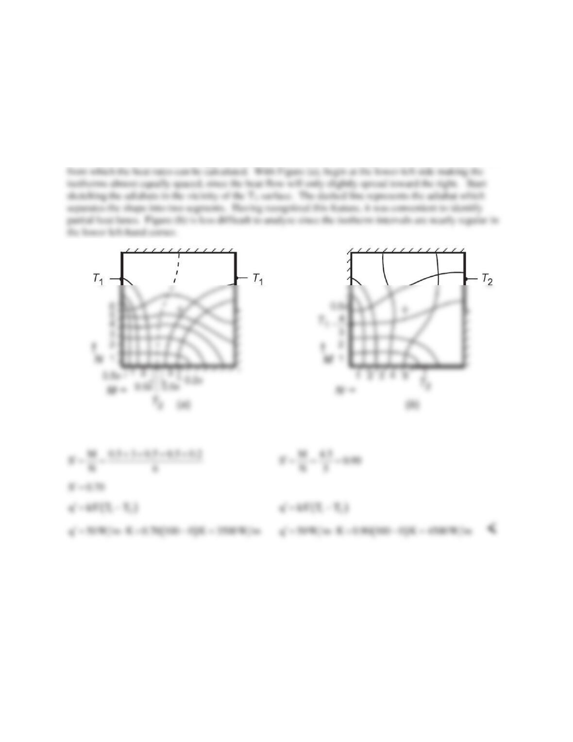
KNOWN: Two–dimensional, square shapes, 1 m to a side, maintained at uniform temperatures as
prescribed, perfectly insulated elsewhere.
FIND: Using the flux plot method, estimate the heat rate per unit length normal to the page if the
thermal conductivity is 50 W/m⋅K
ASSUMPTIONS: (1) Steady-state, two-dimensional conduction, (2) Constant properties.
ANALYSIS: Use the methodology of Section 4S.1 to construct the flux plots to obtain the shape factors
The shape factors are calculated from Equation 4S.7 and the heat rate from Equation 4S.6.
COMMENTS: Using a finite–element package with a fine mesh, we determined heat rates of 4780 and
4575 W/m, respectively, for Figures (a) and (b). The estimate for the less difficult Figure (b) is within
2% of the numerical method result. For Figure (a), our flux plot result was 27% low.