PROBLEM 4.55 (Cont.)
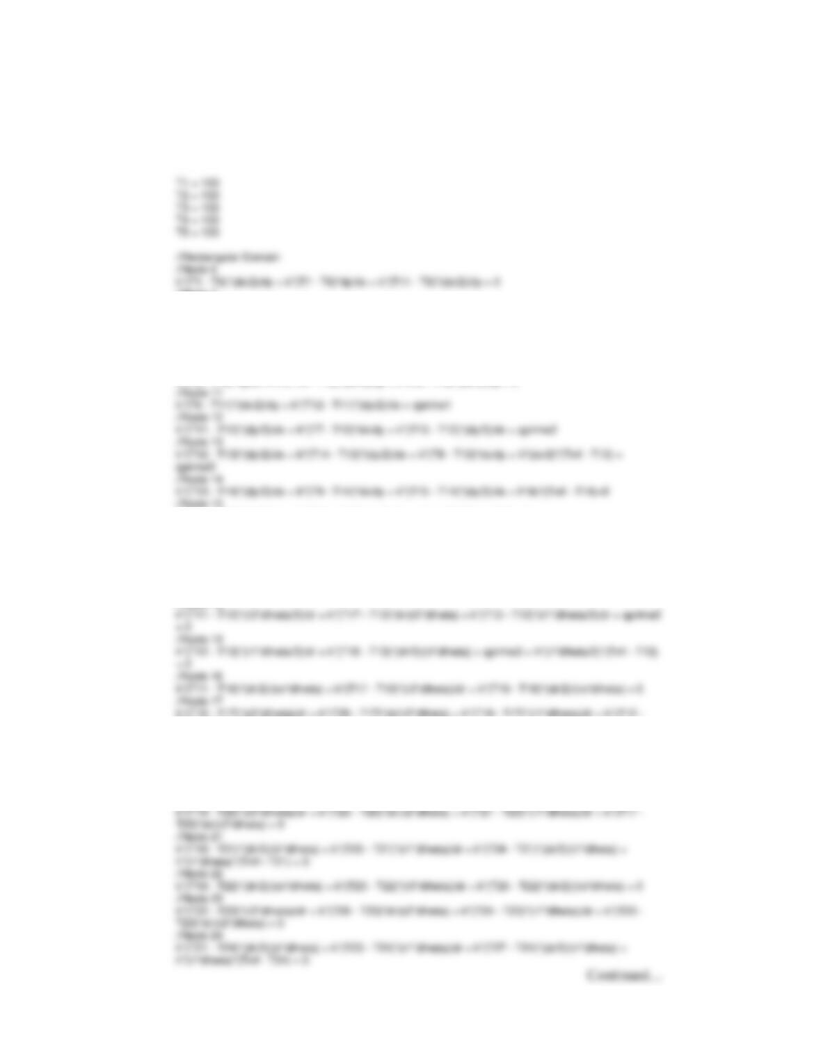
k = 15
h = 240
Tinf = 20
//Node 7
k*(T6 – T7)*dy/dx + k*(T12 – T7)*dx/dy + k*(T8 – T7)*dy/dx + k*(T2 – T7)*dx/dy = 0
//Node 8
k*(T7 – T8)*dy/dx + k*(T13 – T8)*dx/dy + k*(T9 – T8)*dy/dx + k*(T3 – T8)*dx/dy = 0
//Node 9
k*(T8 – T9)*dy/dx + k*(T14 – T9)*dx/dy + k*(T10 – T9)*dy/dx + k*(T4 – T9)*dx/dy = 0
//Node 10
k*(T9 – T10)*dy/dx + k*(T15 – T10)*(dx/2)/dy + k*(T5 – T10)*(dx/2)/dy = 0
k*(T14 – T15)*(dy/2)/dx + k*(T10 – T15)*(dx/2)/dy + h*(dx/2)*(Tinf – T15) = 0
//Cylindrical Domain
//Node 11
k*(T16 – T11)*(dr/2)/(ro*dtheta) + k*(T12 – T11)*(r3*dtheta/2)/dr + qprime1 = 0
//Node 12
T17)*dr/(r2*dtheta) = 0
//Node 18
k*(T13 – T18)*(dr/2)/(ri*dtheta) + k*(T17 – T18)*(r1*dtheta)/dr + k*(T21 – T18)*(dr/2)/(ri*dtheta) +
h*(ri*dtheta)*(Tinf – T18) = 0
//Node 19
k*(T16 – T19)*(dr/2)/(ro*dtheta) + k*(T20 – T19)*(r3*dtheta)/dr + k*(T22 – T19)*(dr/2)/(ro*dtheta) = 0
//Node 20
PROBLEM 4.55 (Cont.)
//Node 25
k*(T22 – T25)*(dr/2)/(ro*dtheta) + k*(T26 – T25)*(r3*dtheta/2)/dr = 0
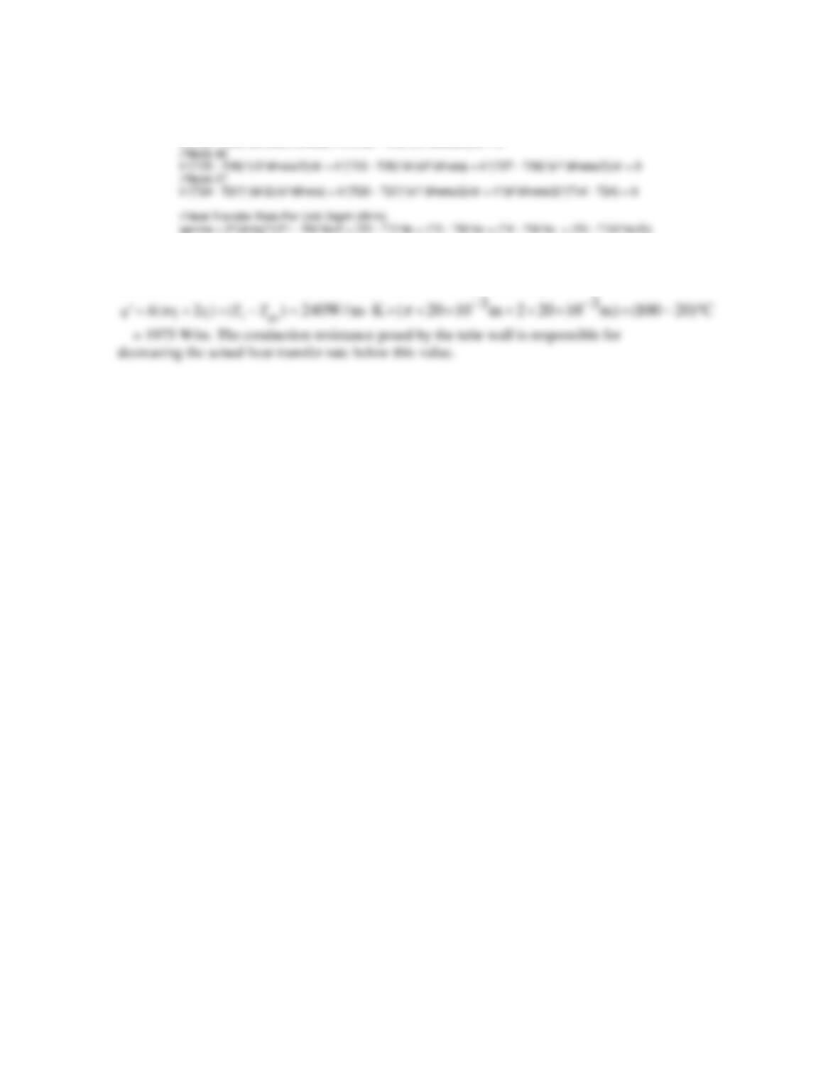
(2) For an isothermal tube at Ts = 100°C, the heat transfer per unit length is
PROBLEM 4.56
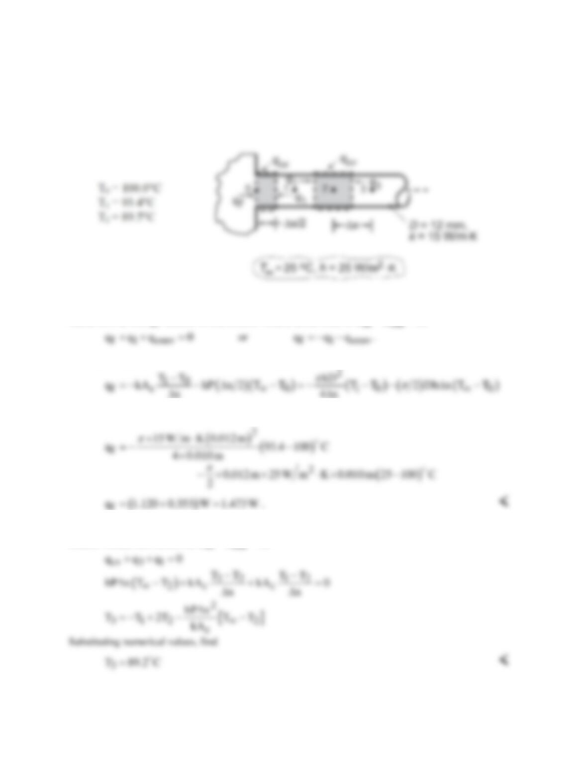
KNOWN: Nodal temperatures from a steady–state finite–difference analysis for a cylindrical fin of
prescribed diameter, thermal conductivity and convection conditions (
T∞
, h).
FIND: (a) The fin heat rate, qf, and (b) Temperature at node 3, T3.
SCHEMATIC:
ASSUMPTIONS: (a) The fin heat rate, qf, is that of conduction at the base plane, x = 0, and can be
found from an energy balance on the control volume about node 0,
EE 0−=
,
Writing the appropriate rate equation for q1 and qconv, with Ac = πD2/4 and P = πD,
Substituting numerical values, with Dx = 0.010 m, find
(b) To determine T3, derive the finite–difference equation for node 3, perform an energy balance on the
control volume shown above,
in out
EE 0−=
,
COMMENTS: Note that in part (a), the convection heat rate from the outer surface of the control
volume is significant (25%). It would have been a poor approximation to ignore this term.
PROBLEM 4.57
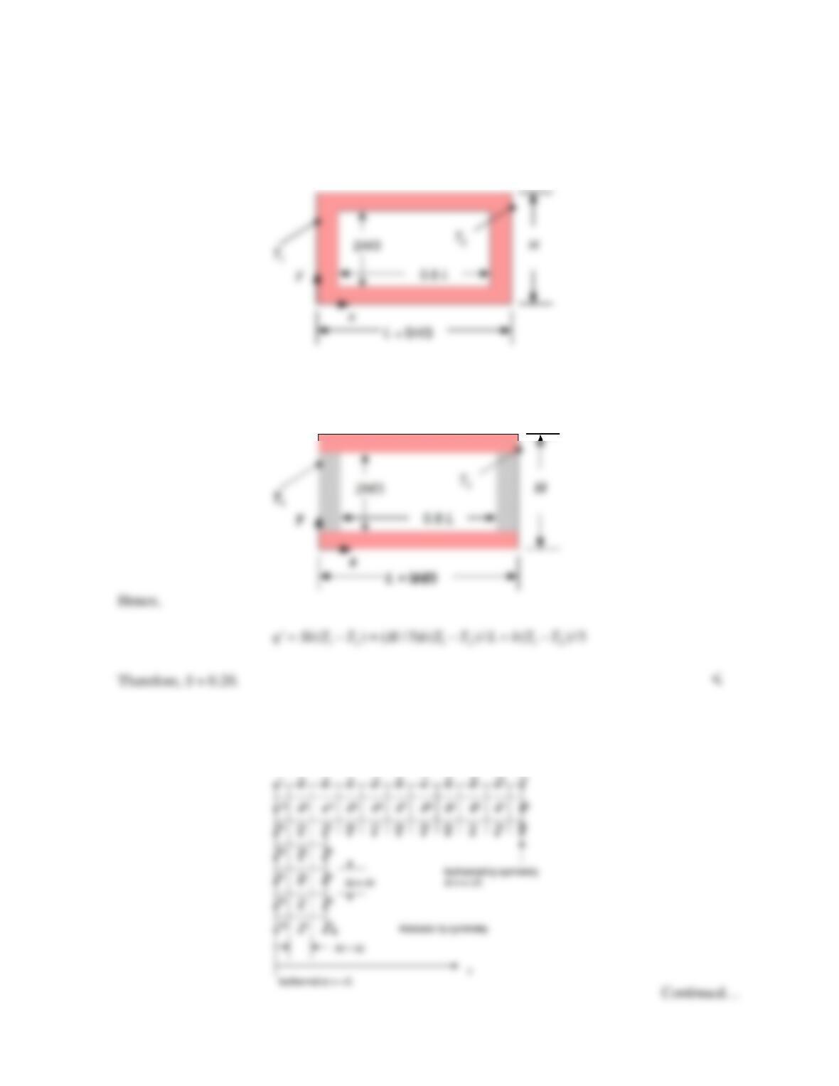
KNOWN: Dimensions of a two-dimensional object with isothermal and adiabatic boundaries.
FIND: (a) Estimate of the shape factor using a one–dimensional analysis and (b) estimate of the shape
factor using a finite difference method with Dx = Dy = 0.05 L.
SCHEMATIC:
ASSUMPTIONS: (1) Steady–state conditions, (2) Constant properties, (3) No internal generation, (4)
One-dimensional conduction in part (a), (5) Two-dimensional conduction in part (b).
ANALYSIS: (a) As a first approximation, we ignore conduction in the cross-hatched regions.
(b) We begin by taking advantage of the symmetry of the problem. Recognize that the line y = H/2 is
an adiabat, and the line x = L/2 is an isotherm at T = (T1 + T2)/2. Hence, only one quarter of the domain
needs to be modeled. Arbitrarily, we select the upper left quarter for analysis. Note that Dx = Dy.
Problem 4.57 (Cont.)
We may use the finite difference equations from the text, or note that for each node, an energy balance
can be written for the corresponding control volume. Consider, for example, the control volume about
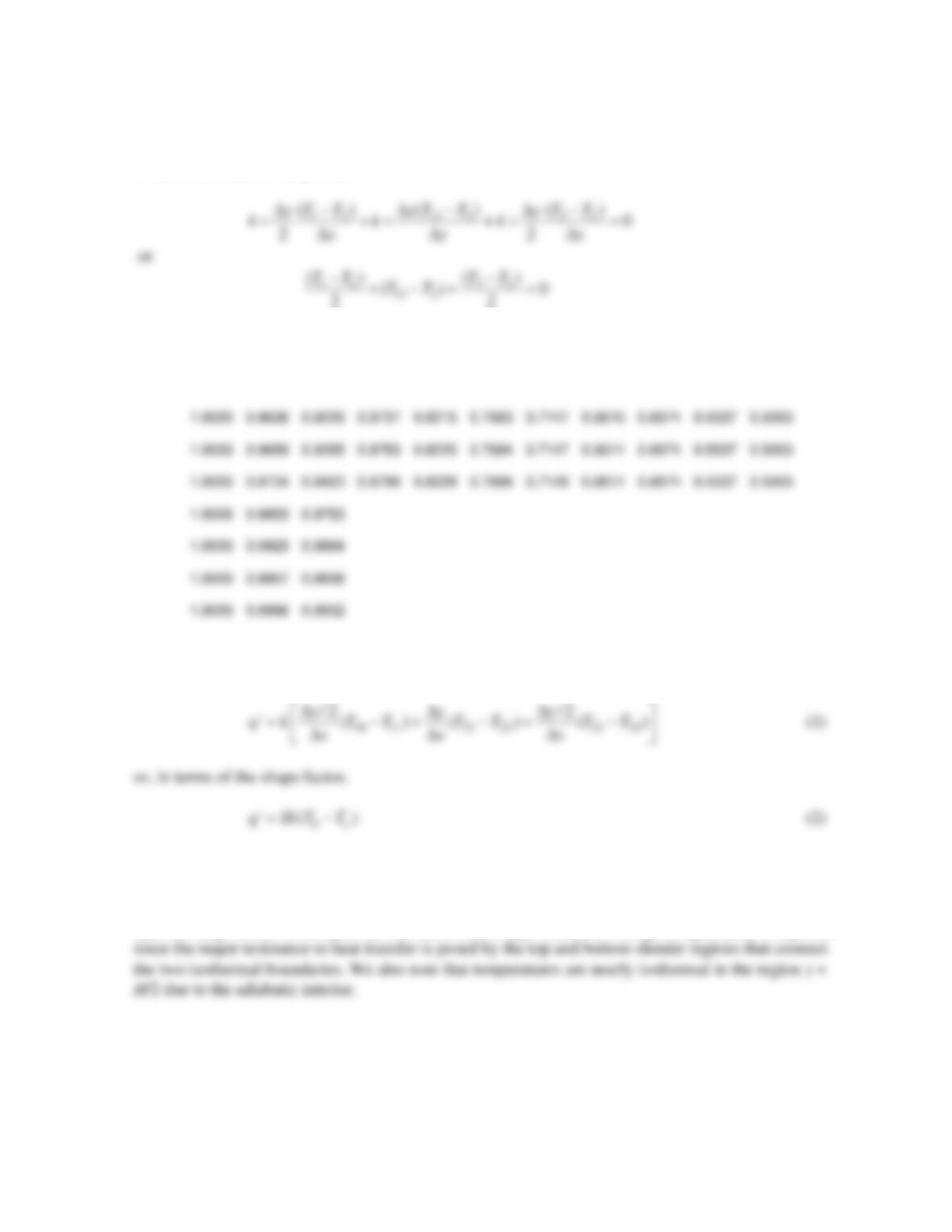
Node 2 for which we may write
We let the temperature at x = 0 be T1 = 1 and the temperature at x = L/2 be T2 = 0.5. The 45 equations
are solved simultaneously with the IHT code provided in the Comment. The resulting nodal
temperatures in the upper left corner are:
After solving for the temperatures, the heat transfer rate per unit depth may be evaluated at any x
location, and for x = L/2 it may be expressed as
Equating Eqs. (1) and (2) yields the shape factor, S ≈ 0.215. <
We note that the shape factor calculated with the finite difference approach is only slightly greater
than the shape factor based upon the one-dimensional approximation. The good agreement is expected
Continued…
Problem 4.57 (Cont.)
COMMENTS: The IHT code is listed below. For each control volume, we note that
0
in
E=
and Dy =
Dx, yielding the following energy balances for all but the isothermal nodes.
Th = 1
Tc =0.5
//Top Row
//Node 1
T1 = Th
//Node 2
(T6 – T7)/2 + (T8 – T7)/2 + (T18 – T7) = 0
//Node 8
(T7 – T8)/2 + (T9 – T8)/2 + (T19 – T8) = 0
//Node 9
(T8 – T9)/2 + (T10 – T9)/2 + (T20 – T9) = 0
(T13 – T14) + (T3 – T14) + (T15 – T14) + (T25 – T14) = 0
//Node 15
(T14 – T15) + (T4 – T15) + (T16 – T15) + (T26 – T15) = 0
//Node 16
(T15 – T16) + (T5 – T16) + (T17 – T16) + (T27 – T16) = 0
//Node 17
(T16 – T17) + (T6 – T17) + (T18 – T17) + (T28 – T17) = 0
//Node 18
(T17 – T18) + (T7 – T18) + (T19 – T18) + (T29 – T18) = 0
//Node 19
Problem 4.57 (Cont.)
(T25 – T26)/2 + (T15 – T26) + (T27 – T26)/2 = 0
//Node 27
(T26 – T27)/2 + (T16 – T27) + (T28 – T27)/2 = 0
//Node 28
T33 = Tc
//Fourth Row from Top
//Node 34
T34 = Th
//Node 35
//Sixth Row from Top
//Node 40
T40 = Th
//Node 41
(T40 – T41) + (T38 – T41) + (T42 – T41) + (T44 – T41) = 0
//Node 42
(T41 – T42) + (T39 – T42)/2 + (T45 – T42)/2 = 0
//Bottom Row
//Node 43
PROBLEM 4.58
KNOWN: Long bar of square cross section, three sides of which are maintained at a constant
temperature while the fourth side is subjected to a convection process.
FIND: (a) The mid–point temperature and heat transfer rate between the bar and fluid; a numerical
technique with grid spacing of 0.2 m is suggested, and (b) Reducing the grid spacing by a factor of 2, find
the midpoint temperature and the heat transfer rate. Also, plot temperature distribution across the surface
exposed to the fluid.
ASSUMPTIONS: (1) Steady-state, two-dimensional conduction, (2) Constant properties.
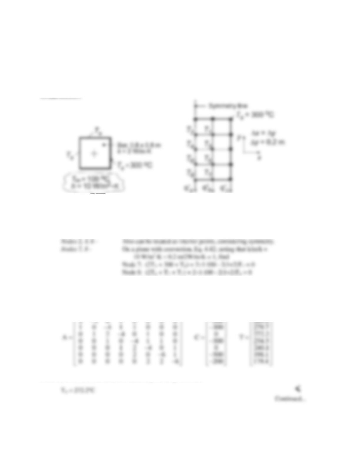
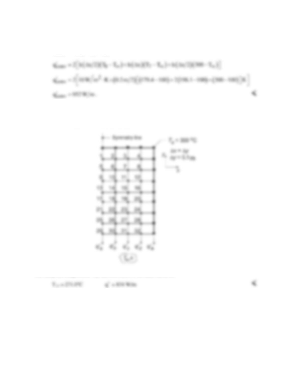
ANALYSIS: (a) Considering symmetry, the nodal network is shown above. The matrix inversion
method of solution will be employed. The finite-difference equations are:
Nodes 1, 3, 5 – Interior nodes, Eq. 4.29; written by inspection.
The solution matrix [T] can be found using a stock matrix program using the [A] and [C] matrices shown
below to obtain the solution matrix [T] (Eq. 4.48). Alternatively, the set of equations could be entered
into the IHT workspace and solved for the nodal temperatures.
4 1 1 0 0 0 0 0 600 292.2
−−
From the solution matrix, [T], find the mid-point temperature as
PROBLEM 4.58 (Cont.)
The heat rate by convection between the bar and fluid is given as,
( )
conv a b c
q 2q q q
′ ′′′
= ++
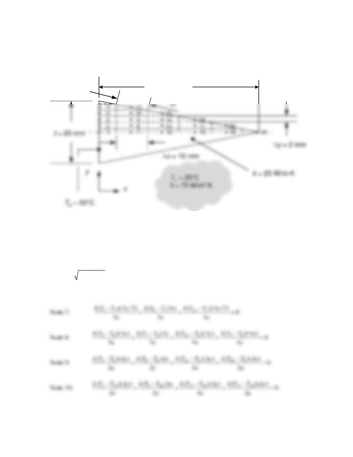
(b) Reducing the grid spacing by a factor of 2, the nodal arrangement will appear as shown. The finite–
difference equation for the interior and centerline nodes were written by inspection and entered into the
IHT workspace. The IHT Finite-Difference Equations Tool for 2-D, SS conditions, was used to obtain
the FDE for the nodes on the exposed surface.
The midpoint temperature T13 and heat rate for the finer mesh are
q′
COMMENTS: The midpoint temperatures for the coarse and finer meshes agree closely, T4 = 272°C
vs. T13 = 271.0°C, respectively. However, the estimate for the heat rate is substantially influenced by the
mesh size;
q′
= 952 vs. 834 W/m for the coarse and finer meshes, respectively.
PROBLEM 4.59
KNOWN: Dimensions of a two-dimensional, straight triangular fin. Fin base and ambient
temperatures, thermal conductivity and heat transfer coefficient.
FIND: Fin efficiency by using a finite difference solution with specified grid.
SCHEMATIC:
L= 50 mm
6
ASSUMPTIONS: (1) Steady–state conditions, (2) Constant properties, (3) No internal generation, (4)
Two–dimensional conduction.
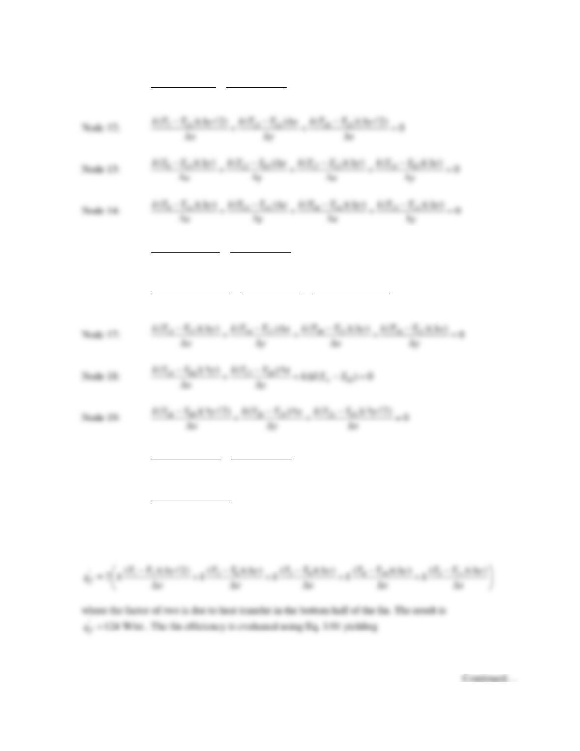
ANALYSIS: We may combine heat fluxes determined from Fourier’s law and Newton’s law of
cooling with expressions for the size of the control surfaces of the various control volumes to
determine the heat rate per unit depth into each control volume within the discretized domain.
Application of conservation of energy for each control volume yields the expression
in
0E=
. Note
that
22
l xyD = D +D
= 10.198 mm.
Nodes 1, 2, 3, 4, 5 and 6: T1 = T2 = T3 = T4 = T5 = T6 = Tb = 50°C.
Continued…
PROBLEM 4.59 (Cont.)
Node 11:
5 11 10 11 11
( )( ) ( ) ( )0
kT T y kT T x h lT T
xy
∞
− D −D
+ +D − =
DD
Node 15:
10 15 14 15 15
( )( ) ( ) ( )0
kT T y kT T x h lT T
xy
∞
− D −D
+ +D − =
DD
Node 16:
12 16 17 16 19 16
()(/2)()()(/2)
0
kT T y kT T x kT T y
xyx
−D −D −D
++ =
DDD
∞
Node 20:
17 20 19 20 20
()()() ( )0
kT T y kT T x h lT T
xy
∞
− D −D
+ +D − =
DD
Node 21:
( )
19 21 21
( )( / 2) /2 ( ) 0
kT T y hl T T
x
∞
−D+D − =
D
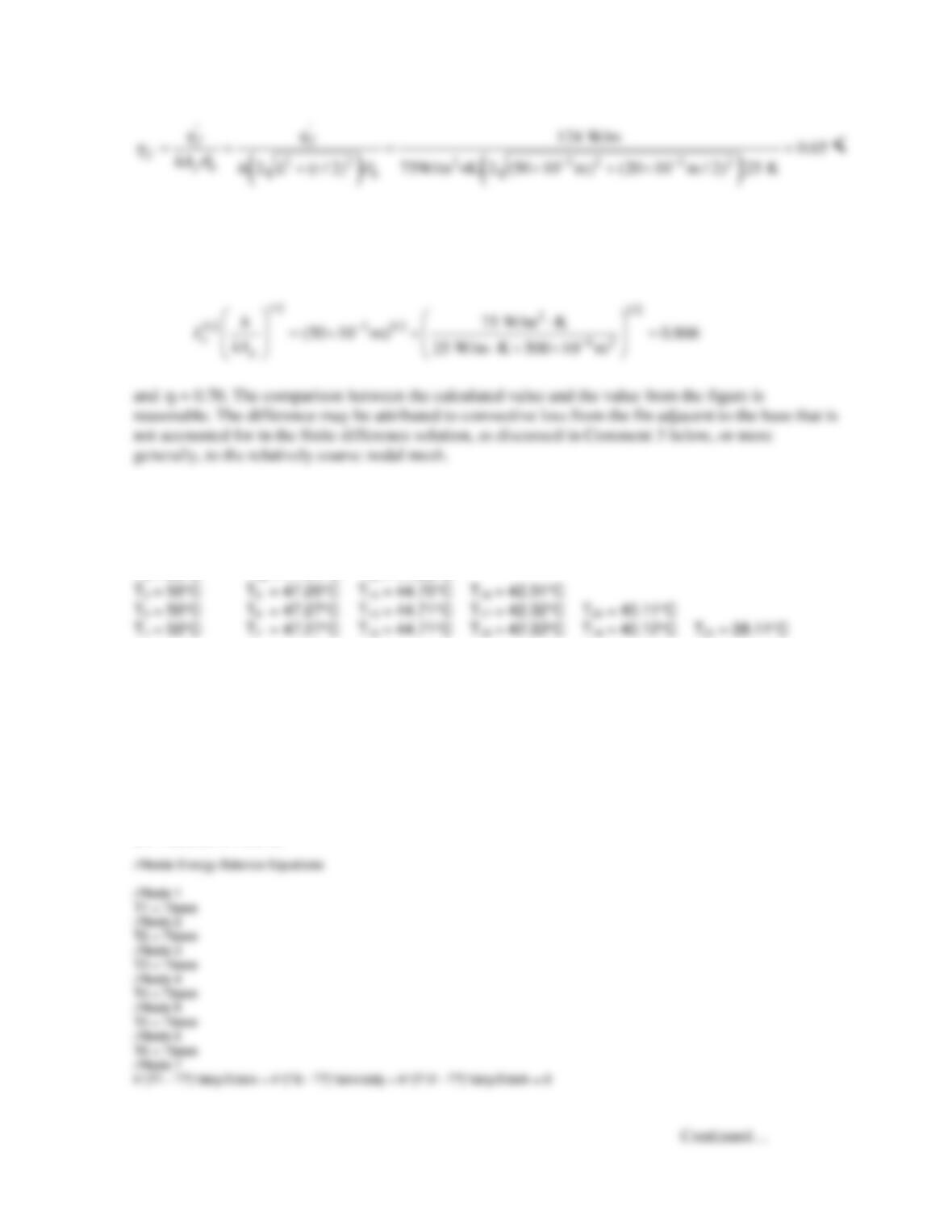
The fin heat rate per unit length is evaluated by considering conduction into its base expressed as
PROBLEM 4.59 (Cont.)
From Fig. 3.19 we find Lc = 50 × 10-3 m, Ap = Lt/2 = (50 × 10-3 m × 20 × 10-3 m)/2 = 500 × 10-6 m2.
Therefore,
COMMENTS: (1) The nodal temperatures are:
T6 = 50°C
T5 = 50°C T11 = 47.22°C
T4 = 50°C T10 = 47.24°C T15 = 44.68°C
Note the nearly uniform cross-sectional temperatures within the fin. Temperatures near the
centerline are only slightly warmer than corresponding temperatures at a particular x–location
nearer to the convectively–cooled fin surface. (2) The IHT code is listed below.
// Input Parameters
k = 25
Tinf = 25
Tbase = 50
delx = 0.01
dely = 0.002
h = 75
dell = sqrt(delx^2 + dely^2)
PROBLEM 4.59 (Cont.)
//Node 8
k*(T2 – T8)*dely/delx + k*(T7 – T8)*delx/dely + k*(T13 – T8)*dely/delx + k*(T9 – T8)*delx/dely = 0
//Node 9
k*(T3 – T9)*dely/delx + k*(T8 – T9)*delx/dely + k*(T14 – T9)*dely/delx + k*(T10 – T9)*delx/dely = 0
//Node 15
k*(T10 – T15)*dely/delx + k*(T14 – T15)*delx/dely + h*dell*(Tinf – T15) = 0
//Node 16
k*(T12 – T16)*dely/2/delx + k*(T17 – T16)*delx/dely + k*(T19 – T16)*dely/2/delx = 0
//Node 17
k*(T13 – T17)*dely/delx + k*(T16 – T17)*delx/dely + k*(T20 – T17)*dely/delx + k*(T18 – T17)*delx/dely = 0
//Node 18
k*(T14 – T18)*dely/delx + k*(T17 – T18)*delx/dely + h*dell*(Tinf – T18) = 0
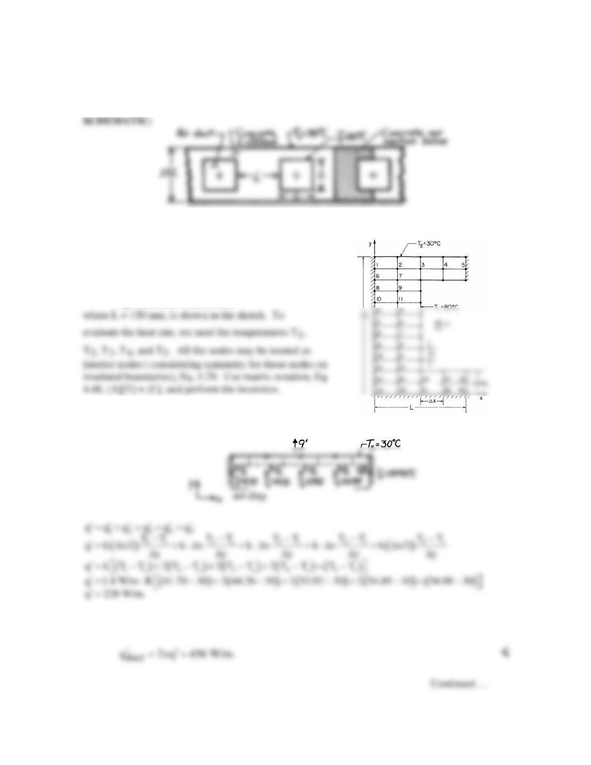
(3) The finite difference equations do not account for convective losses from the fin in the exposed
region of length
/2lD
adjacent to the root of the fin. If this convective loss is estimated to be
PROBLEM 4.60
KNOWN: Rectangular air ducts having surfaces at 80°C in a concrete slab with an insulated bottom
and upper surface maintained at 30°C.
FIND: Heat rate from each duct per unit length of duct,
q.
′
ASSUMPTIONS: (1) Steady-state conditions, (2) Two-dimensional conduction, (3) No internal
volumetric generation, (4) Constant properties.
PROPERTIES: Concrete (given): k = 1.4 W/m⋅K.
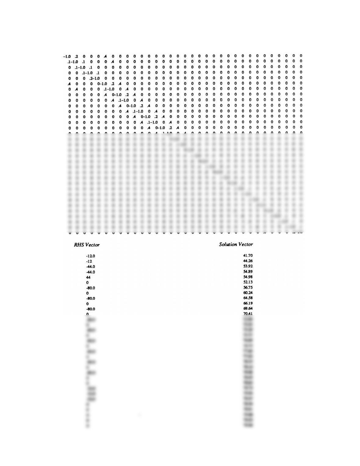
ANALYSIS: Taking advantage of symmetry, the
nodal network, using the suggested grid spacing
Dx = 2Dy = 37.50 mm
Dy = 0.125L = 18.75 mm
The heat rate per unit length from the prescribed section of
the duct follows from an energy balance on the nodes at the
top isothermal surface.
Since the section analyzed represents one-half of the region about an air duct, the heat loss per unit
length for each duct is,
PROBLEM 4.60 (Cont.)
Coefficient matrix [A]
PROBLEM 4.61
KNOWN: Bar of known thermal conductivity and trapezoidal cross section. Temperatures of left and
right faces.
FIND: Heat transfer rate per unit bar length using Dx = Dy = 10 mm. Compare to heat rate for
rectangular cross section.
SCHEMATIC:
ASSUMPTIONS: (1) Steady-state conditions, (2) Uniform properties, (3) No internal heat generation,
(4) Two–dimensional conduction.
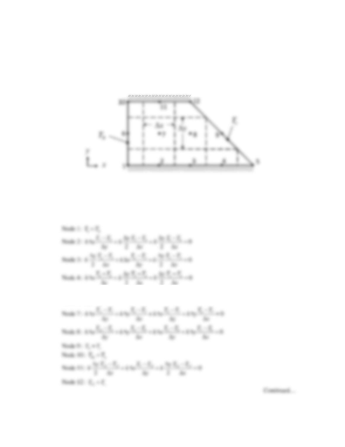
ANALYSIS: The discretized solution domain is shown in the schematic. The finite difference equations
are:
5
Node 5:
c
TT=
6
Node 6 :
h
TT=
PROBLEM 4.61 (Cont.)
Solving the preceding equations yields
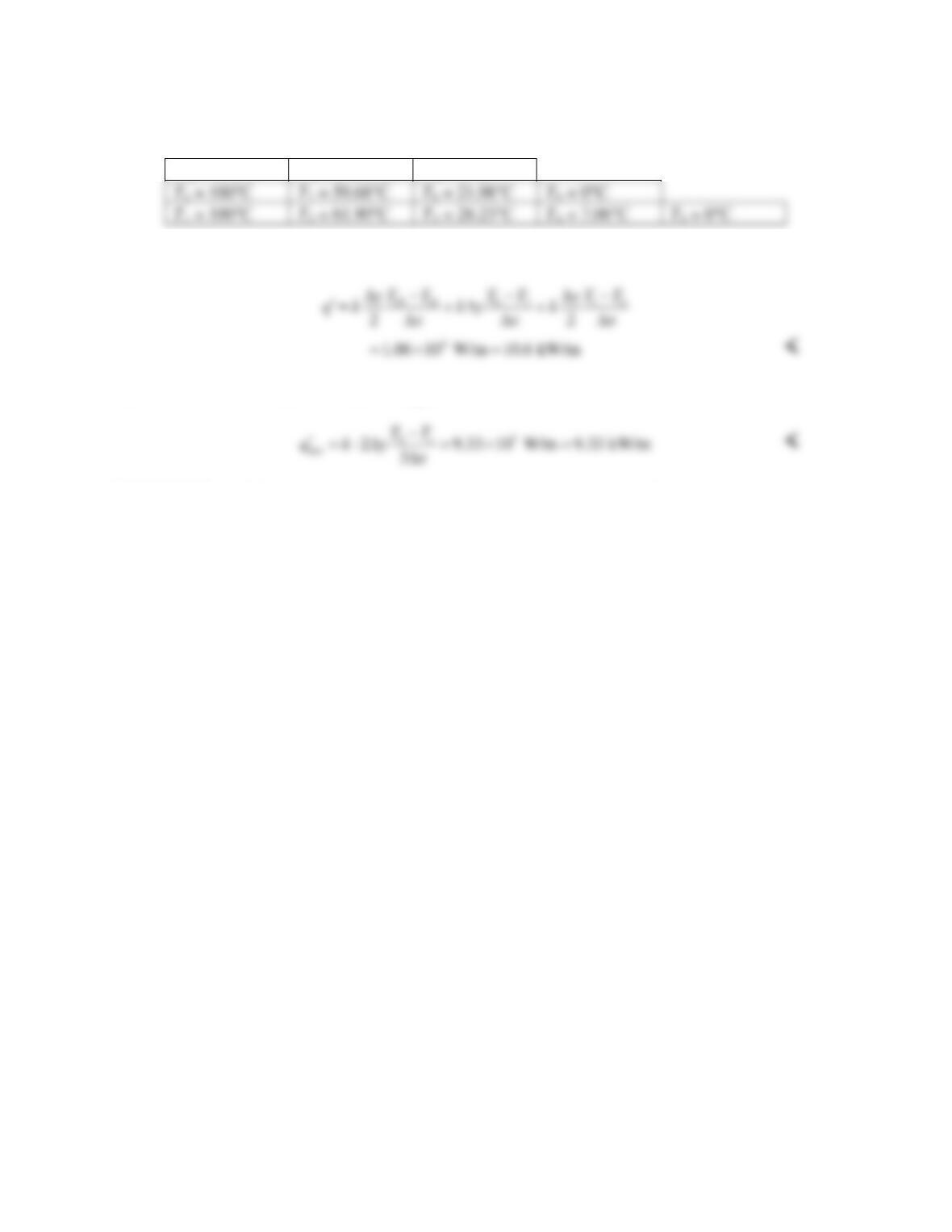
T10 = 100°C
T11 = 54.84°C
T12 = 0°C
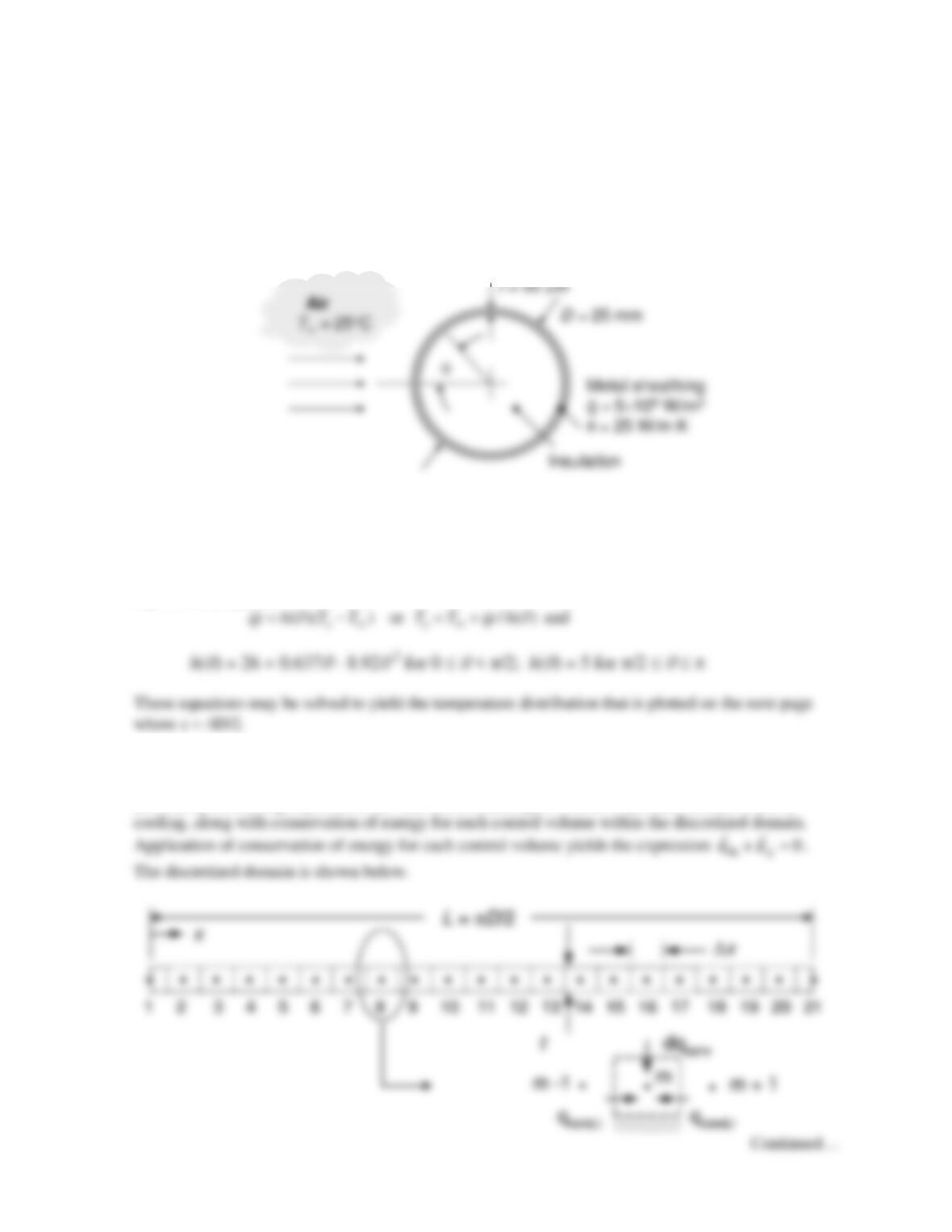
The heat rate per unit length may be calculated as
The heat rate for the 20 mm × 30 mm rectangular cross section bar is
COMMENTS: (1) The trapezoidal and rectangular bars are of the same mass. Hence, the trapezoidal bar
has a greater heat transfer rate per unit mass. (2) The heat rate per unit length can be calculated in various
ways. For example, it could be determined by calculating the heat rate in the horizontal direction per unit
length between nodes 11 and 12, 7 and 8, plus that between nodes 2 and 3.
T1 = 100°C
T2 = 61.90°C
T3 = 28.23°C
T4 = 7.06°C
T5 = 0°C
PROBLEM 4.62
KNOWN: Dimensions of long cylinder, thickness of metal sheathing, volumetric generation rate
within the sheathing, thermal conductivity of sheathing and convection heat transfer coefficient
dependence upon angle
θ
.
FIND: (a) Temperature distribution within the thin sheathing neglecting
θ
–direction conduction heat
transfer, (b) temperature distribution in the sheathing accounting for
θ
-direction conduction heat
transfer in the metal.
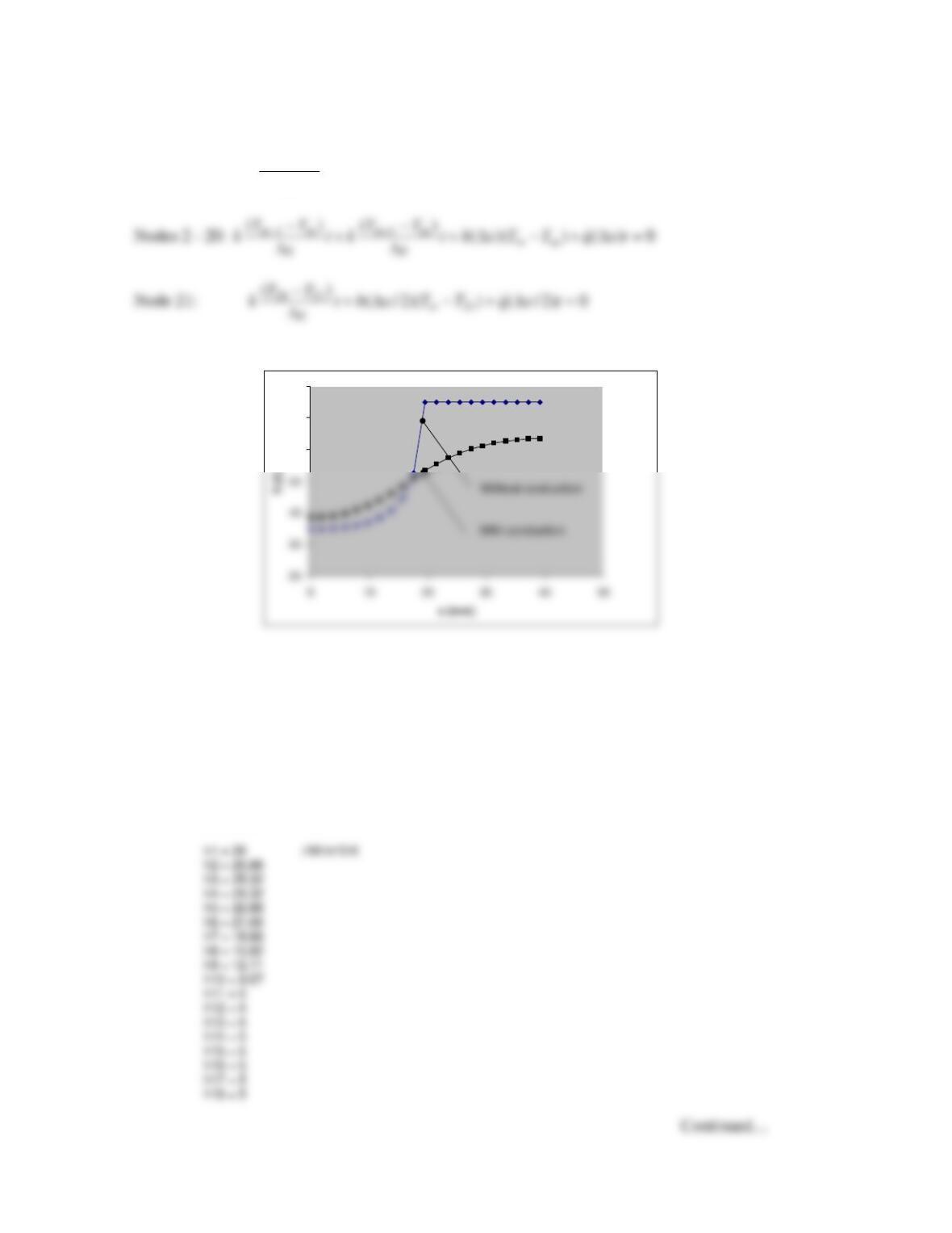
SCHEMATIC:
ASSUMPTIONS: (1) Steady–state conditions, (2) Constant properties, (3) Uniform internal
generation, (4) Metal sheathing is very thin relative to cylinder diameter, (5) One-dimensional
conduction, (6) Negligible radiation.
ANALYSIS: (a) Neglecting conduction in the
θ
–direction in the sheathing, an energy balance at
any
θ
location yields
(b) Since the sheathing is thin relative to the cylinder diameter, we may evaluate one–dimensional
conduction in the x–direction using the Cartesian coordinate system. The finite difference equations are
derived by combining expressions for heat fluxes based upon Fourier’s law and Newton’s law of
PROBLEM 4.62 (Cont.)
The finite difference equations are as follows.
Node 1:
21 1
()
( / 2)( ) ( / 2) 0
TT
k thx T T qx t
x∞
−+D − +D =
D
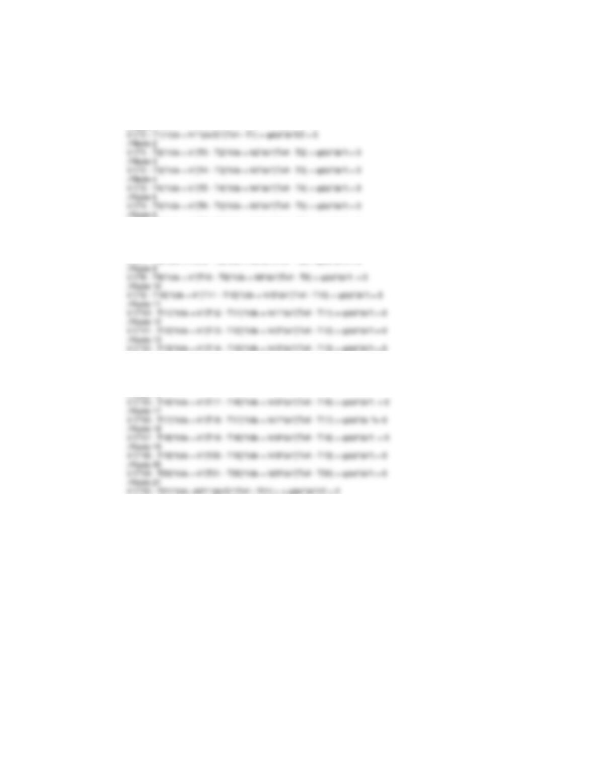
The temperature distribution is plotted below.
COMMENTS: (1) Conduction in the
θ
-direction within the sheathing smears the temperature
distribution, increasing the low temperatures on the upstream half of the cylinder and lowering
the temperatures on the downstream half of the cylinder. (2) The IHT code is listed below.
qdot = 5*10^6 //W/m^3
t = 50*10^(–6) //m
Tinf = 25 + 273 //K
k = 25 //W/m⋅K
D = 25/1000 //m
L = pi*D/2 //m
dx = L/20 //m
60
70
80
60
70
80
PROBLEM 4.62 (Cont.)
h19 = 5
h20 = 5
h21 = 5
//Node 1
k*(T5 – T6)*t/dx + k*(T7 – T6)*t/dx + h6*dx*(Tinf – T6) + qdot*dx*t = 0
//Node 7
k*(T6 – T7)*t/dx + k*(T8 – T7)*t/dx + h7*dx*(Tinf – T7) + qdot*dx*t = 0
//Node 8
k*(T7 – T8)*t/dx + k*(T9 – T8)*t/dx + h8*dx*(Tinf – T8) + qdot*dx*t = 0
//Node 14
k*(T13 – T14)*t/dx + k*(T15 – T14)*t/dx + h14*dx*(Tinf – T14) + qdot*dx*t = 0
//Node 15
k*(T14 – T15)*t/dx + k*(T16 – T15)*t/dx + h15*dx*(Tinf – T15) + qdot*dx*t = 0
//Node 16