PROBLEM 4.63
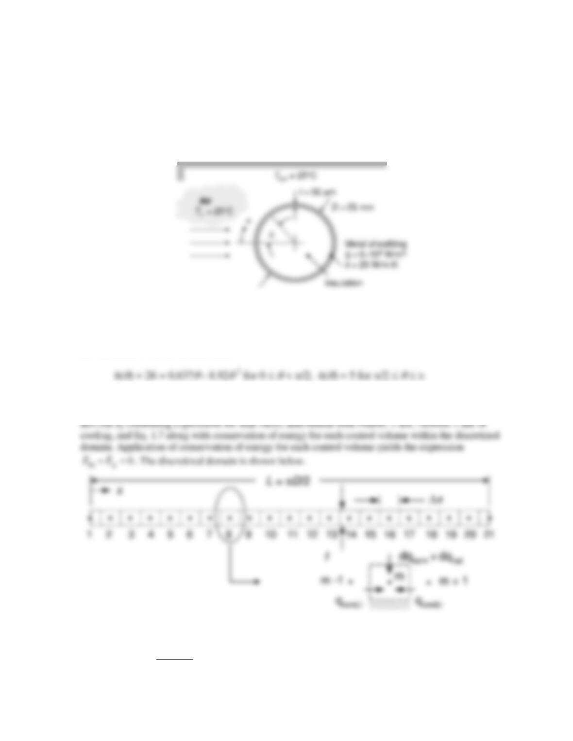
KNOWN: Diameter of long cylinder, thickness of metal sheathing, volumetric generation rate within
the sheathing, thermal conductivity of sheathing and convection heat transfer coefficient dependence
upon angle
q
. Emissivity of the sheathing.
FIND: (a) Temperature distribution within the thin sheathing accounting for convection, conduction
in the sheathing, and radiation exchange with the surroundings.
SCHEMATIC:
ASSUMPTIONS: (1) Steady–state conditions, (2) Constant properties, (3) Uniform internal
generation, (4) Metal sheathing is very thin relative to cylinder diameter, (5) One-dimensional
conduction, (6) Large surroundings.
ANALYSIS: From Problem 4.62,
Since the sheathing is thin relative to the cylinder diameter, we may evaluate one–dimensional
conduction in the x–direction using the Cartesian coordinate system. The finite difference equations are
Energy balances for the control volumes are as follows.
Node 1:
44
21 1 sur 1
()
( / 2)( ) ( / 2)( ) ( / 2) 0
TT
k thxTT xTT qxt
x
εs
∞
−+∆ − + ∆ − +∆ =
∆
Continued…
PROBLEM 4.63 (Cont.)
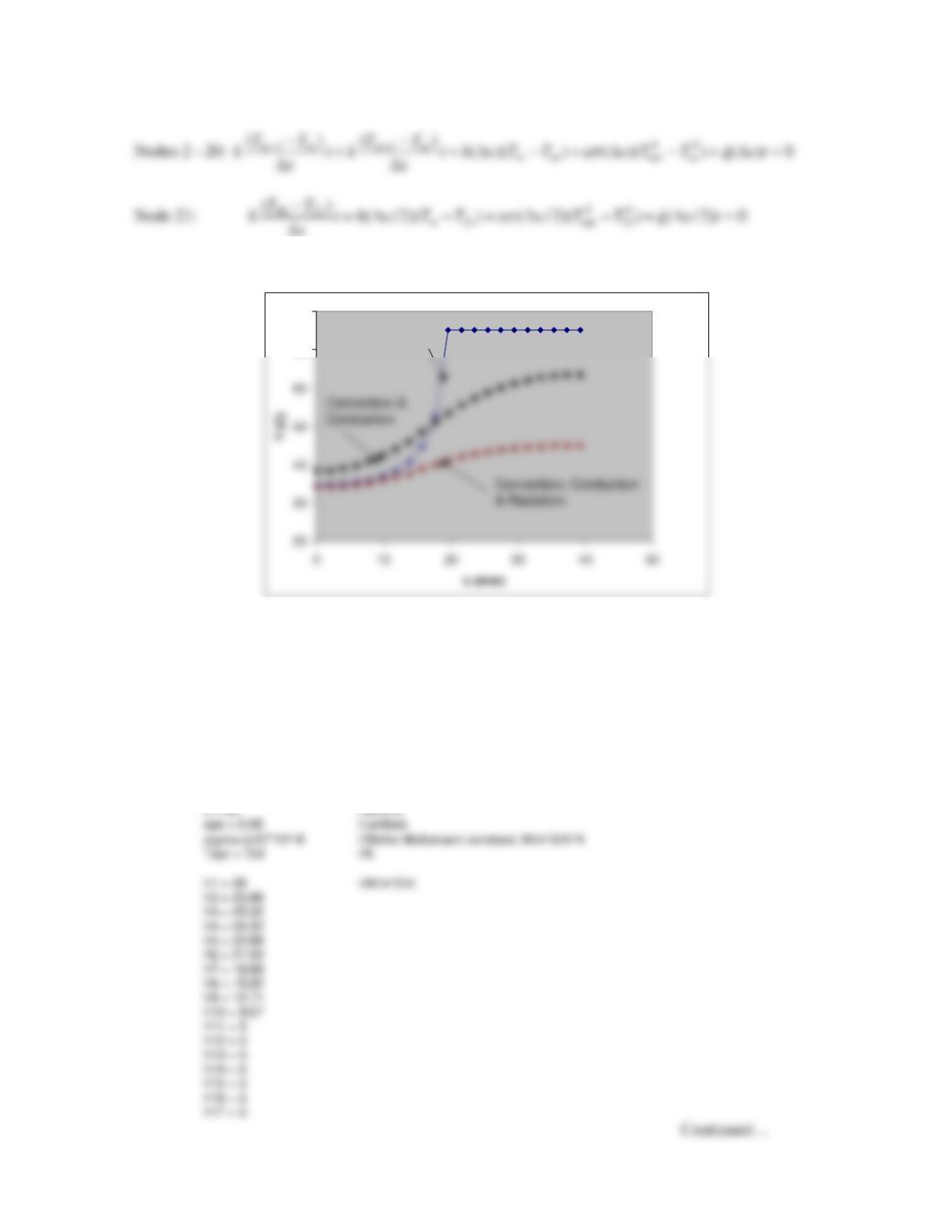
The temperature distribution is plotted below.
COMMENTS: (1) Inclusion of radiation in the analysis shows that the resulting
temperatures are reduced overall, as expected. The effects of conduction and radiation on
local temperatures are comparable. (2) The IHT code is listed below.
D = 25/1000 //m
L = pi*D/2 //m
dx = L/20 //m
qdot = 5*10^6 //W/m^3
t = 50*10^(–6) //m
Tinf = 25 + 273 //K
70
80
Convection only
70
80
Convection only
PROBLEM 4.63 (Cont.)
h18 = 5
h19 = 5
h20 = 5
//Node 9
k*(T8 – T9)*t/dx + k*(T10 – T9)*t/dx + h9*dx*(Tinf – T9) + eps*sigma*dx*(Tsur^4 – T9^4) + qdot*dx*t = 0
//Node 10
k*(T9 – T10)*t/dx + k*(T11 – T10)*t/dx + h10*dx*(Tinf – T10) + eps*sigma*dx*(Tsur^4 – T10^4) +
qdot*dx*t = 0
//Node 11
k*(T10 – T11)*t/dx + k*(T12 – T11)*t/dx + h11*dx*(Tinf – T11) + eps*sigma*dx*(Tsur^4 – T11^4) +
qdot*dx*t = 0
//Node 12
k*(T11 – T12)*t/dx + k*(T13 – T12)*t/dx + h12*dx*(Tinf – T12) + eps*sigma*dx*(Tsur^4 – T12^4) +
qdot*dx*t = 0
//Node 13
k*(T12 – T13)*t/dx + k*(T14 – T13)*t/dx + h13*dx*(Tinf – T13) + eps*sigma*dx*(Tsur^4 – T13^4) +
qdot*dx*t = 0
PROBLEM 4.64
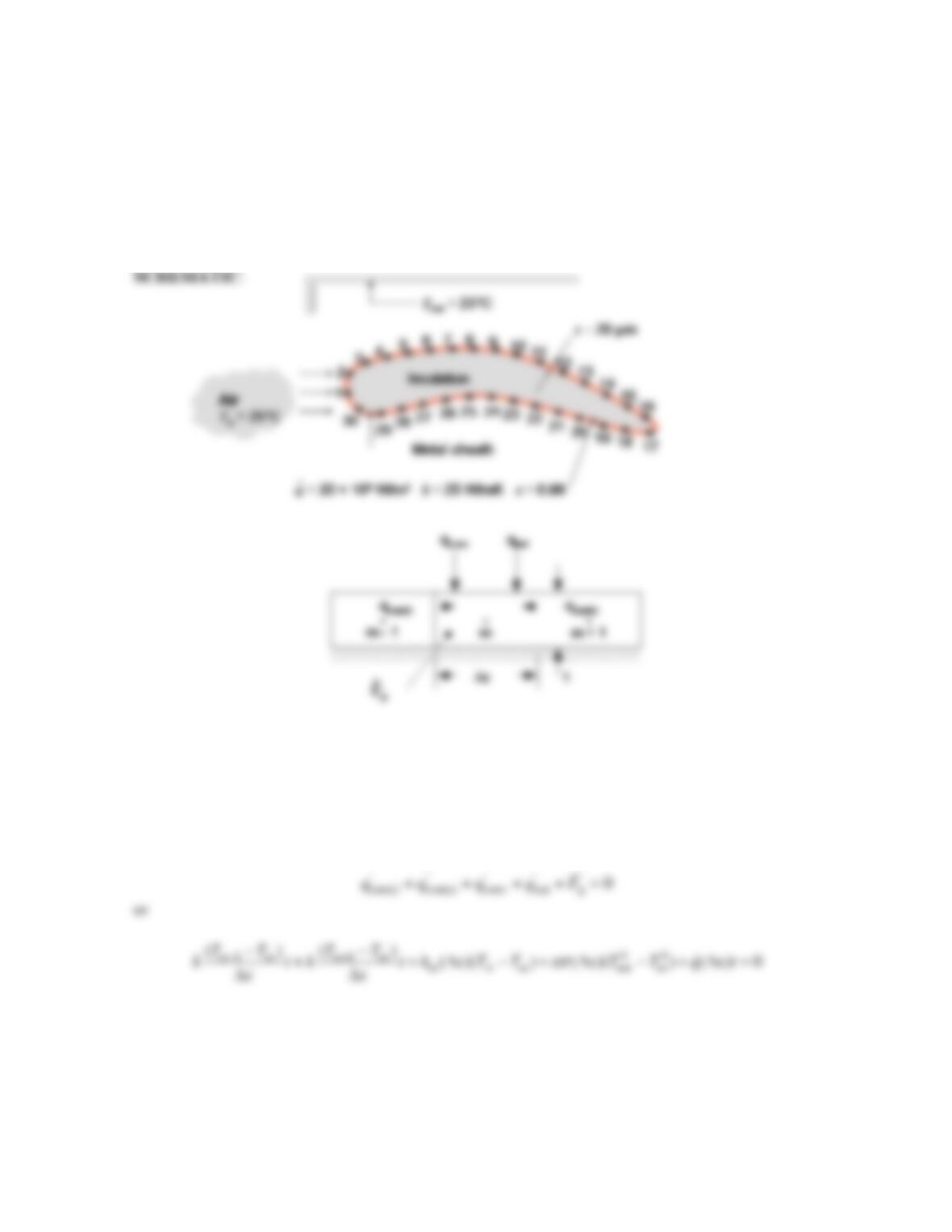
KNOWN: Geometry of long airfoil shape, thickness of metal sheathing, volumetric generation rate
within the sheathing, thermal conductivity of sheathing, emissivity of the sheathing, and measured
temperatures at discrete locations.
FIND: Local convection coefficient at discrete locations accounting for conduction along the
sheathing and radiation. Determine effects of conduction and radiation on the calculated convection
heat transfer coefficients.
ASSUMPTIONS: (1) Steady–state conditions, (2) Constant properties, (3) Uniform internal
generation, (4) Metal sheathing is very thin relative to cylinder diameter, (5) One-dimensional
conduction, (6) Large surroundings.
ANALYSIS: We apply Newton’s law of cooling, Fourier’s law and Eq. 1.7 to a general control
volume about the thin sheathing to find the following general finite-difference formula.
Recognizing that for m = 1, m – 1 = 30, we may substitute values of Tm – 1, Tm, and Tm + 1 and ∆x = 2
mm into the preceding formula and solve for hm. The results for case A (inclusion of convection,
conduction and radiation), case B (inclusion of convection and conduction only) and case C (inclusion
of convection only) are tabulated below.
Continued…
PROBLEM 4.64 (Cont.)
m Tm (°C) hm,A (W/m2⋅K) hm,B (W/m2⋅K) hm,C (W/m2⋅K)
1 27.77 162.8 168.8 144.4
2 27.67 150.4 156.4 149.8
10 32.18 59.88 65.98 55.71
11 34.29 42.01 48.17 43.06
12 36.78 27.93 34.17 33.96
13 39.29 19.14 25.45 27.99
14 41.51 9.89 16.28 24.23
15 42.68 9.06 15.48 22.62
16 42.84 4.01 10.44 22.42
17 41.29 3.98 10.36 24.55
Note: Maximum predicted values are underlined, while minimum predicted values are italicized.
COMMENTS: (1) The heat transfer coefficient distribution is non-uniform. Such non-uniformity is
typical of situations involving convection around complex geometries. The largest heat transfer
PROBLEM 4.65
KNOWN: Bar of rectangular cross-section subjected to prescribed boundary conditions.
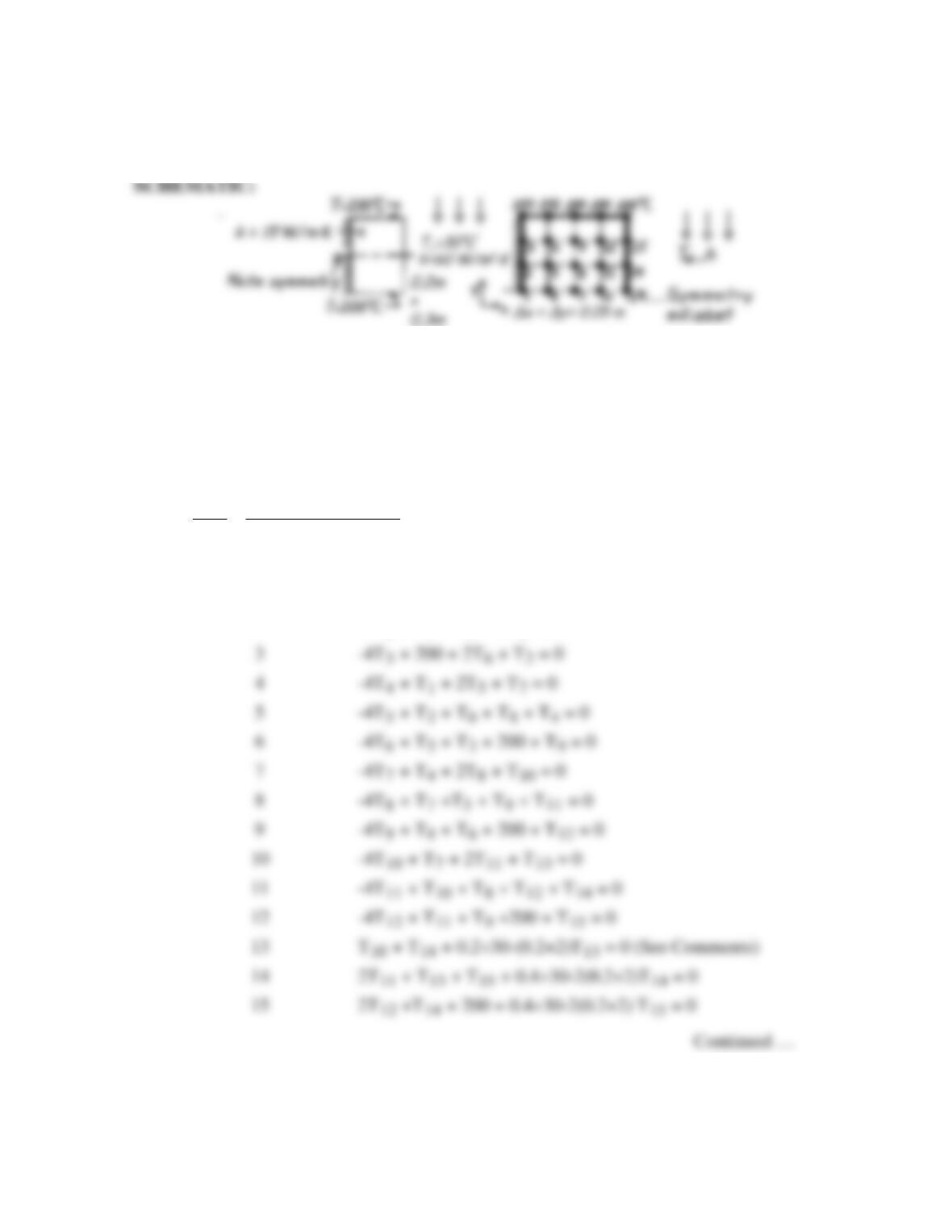
FIND: Using a numerical technique with a grid spacing of 0.05 m, determine the temperature
distribution and the heat transfer rate from the bar to the fluid.
ASSUMPTIONS: (1) Steady-state conditions, (2) Two-dimensional conduction, (3)
Constant properties.
ANALYSIS: The nodal network has ∆x = ∆y = 0.05m. Note the adiabat corresponding to
system symmetry. The finite–difference equations for each node can be written using either
Eq. 4.29, for interior nodes, or Eq. 4.42 (or 4.43), for a plane surface with convection. In the
case of adiabatic surfaces, Eq. 4.42 (or 4.43) is used with h = 0. Note that
2
h x 60W/m K 0.05m 0.2.
k 15 W/m K
∆ ⋅×
= =
⋅
Node Finite-Difference Equations
1 -2T1 + T2 + T4 = 0
2 -4T2 + T1 + T3 + 2T5 = 0
PROBLEM 4.65 (Cont.)
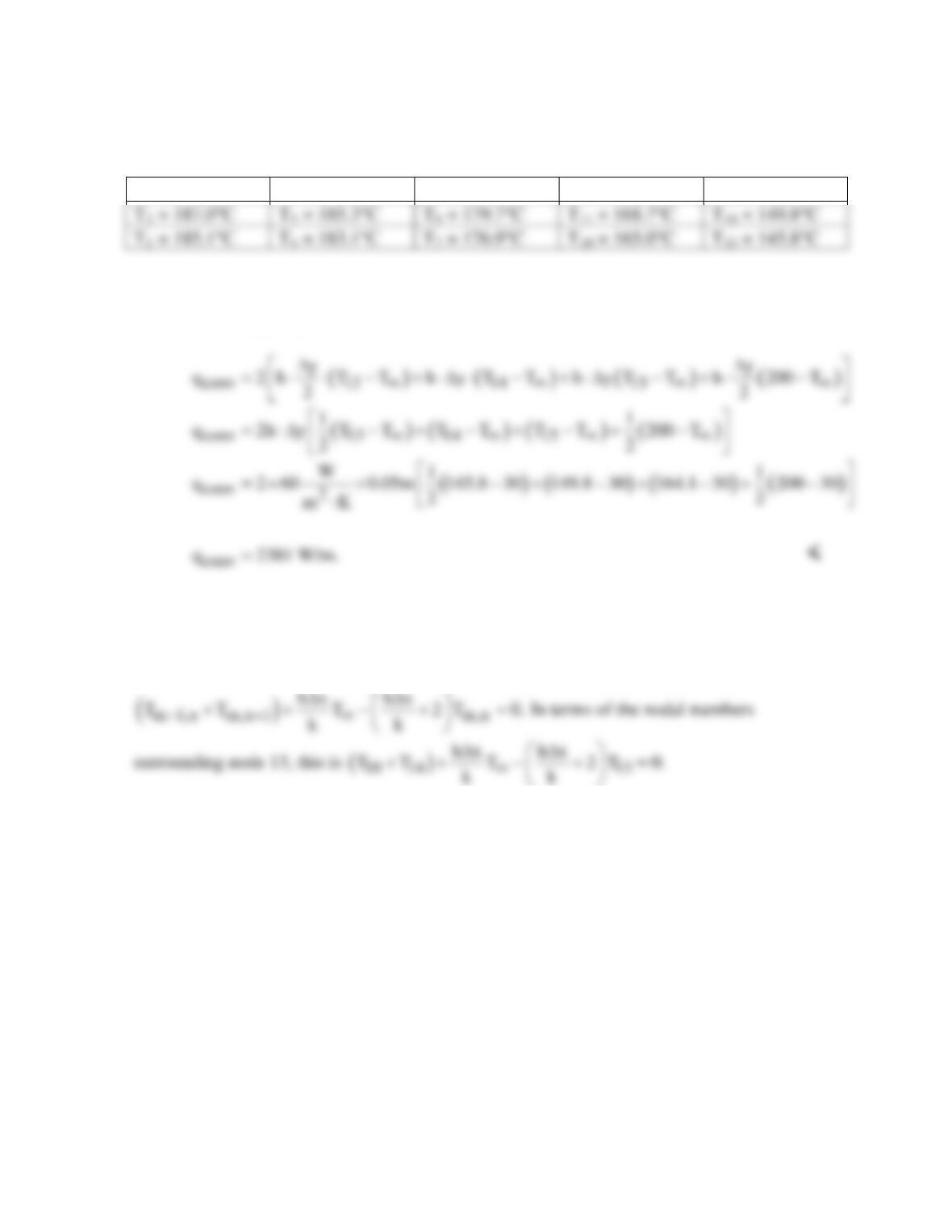
Solving the preceding equations simultaneously using IHT or a calculator or other software
tool yields
T3 = 192.5°C
T6 = 191.4°C
T9 = 187.8°C
T12 = 180.1°C
T15 = 164.1°C
Considering symmetry, the heat transfer rate to the fluid is twice the convection rate from the surfaces
of the control volumes exposed to the fluid. Using Newton’s law of cooling, considering a unit
thickness of the bar, find
COMMENTS: The finite difference equation for node 13 may be obtained from a modified form of
Eq. 4.42. Referring to the figure for Case 3 of Table 4.2, the horizontal line joining nodes m-1,n and
m,n is a symmetry plane for the situation of node 13. Therefore, Tm-1,n = Tm+1,n . Using this substitution
in Eq. 4.42 (and dividing the equation by 2) results in
T2 = 187.0°C
T5 = 185.3°C
T8 = 179.7°C
T11 = 168.7°C
T14 = 149.8°C
T1 = 185.1°C
T4 = 183.1°C
T7 = 176.9°C
T10 = 165.0°C
T13 = 145.8°C
PROBLEM 4.66
KNOWN: Upper surface and grooves of a plate are maintained at a uniform temperature T1, while the
lower surface is maintained at T2 or is exposed to a fluid at T∞.
FIND: (a) Heat rate per width of groove spacing (w) for isothermal top and bottom surfaces using a
finite–difference method with ∆x = 40 mm, (b) Effect of grid spacing and convection at bottom surface.
SCHEMATIC:
ASSUMPTIONS: (1) Steady-state, two-dimensional conduction, (2) Constant properties.
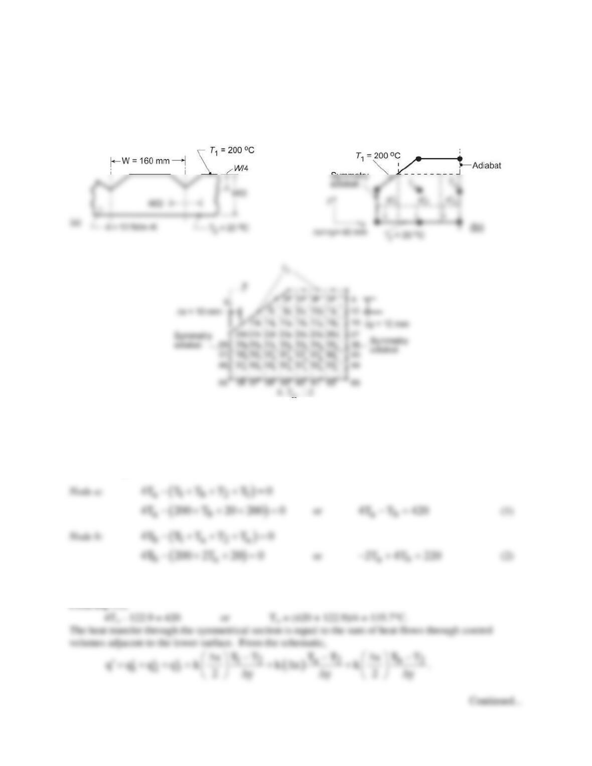
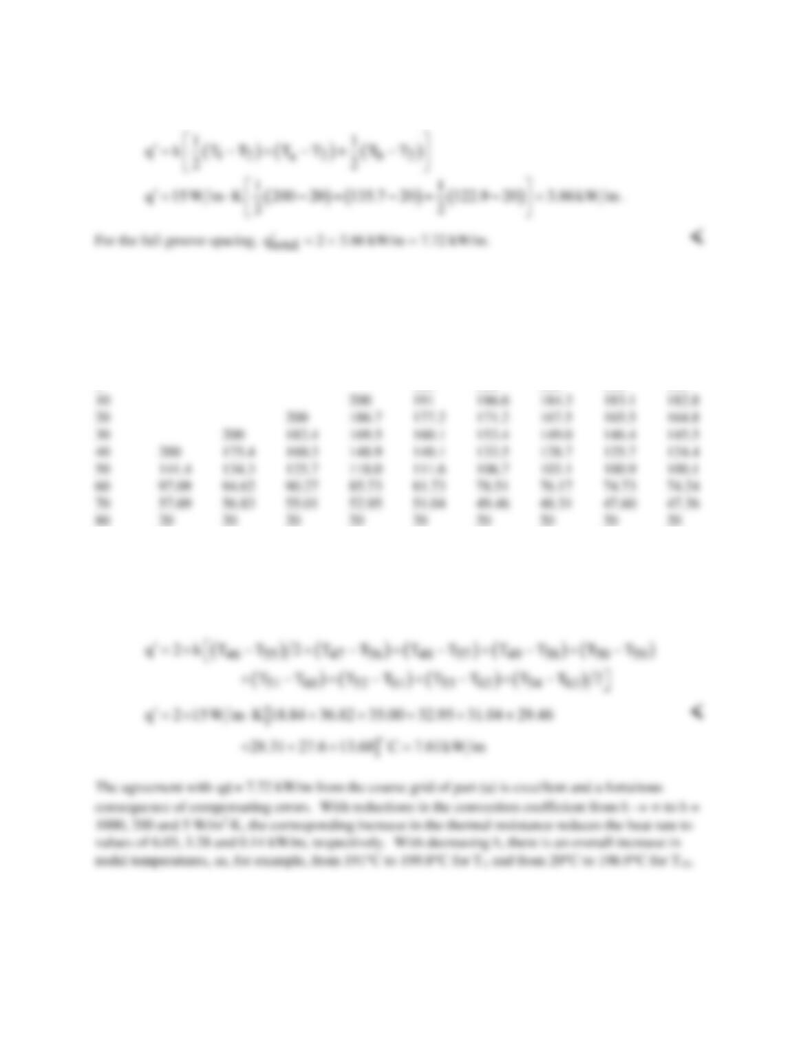
ANALYSIS: (a) Using a space increment of ∆x = 40 mm, the symmetrical section shown in schematic
(b) corresponds to one-half the groove spacing. There exist only two interior nodes for which finite-
difference equations must be written.
Multiply Eq. (2) by 2 and add to Eq. (1) to obtain
7Tb = 860 or Tb = 122.9°C
PROBLEM 4.66 (Cont.)
Noting that ∆x = ∆y, regrouping and substituting numerical values, find
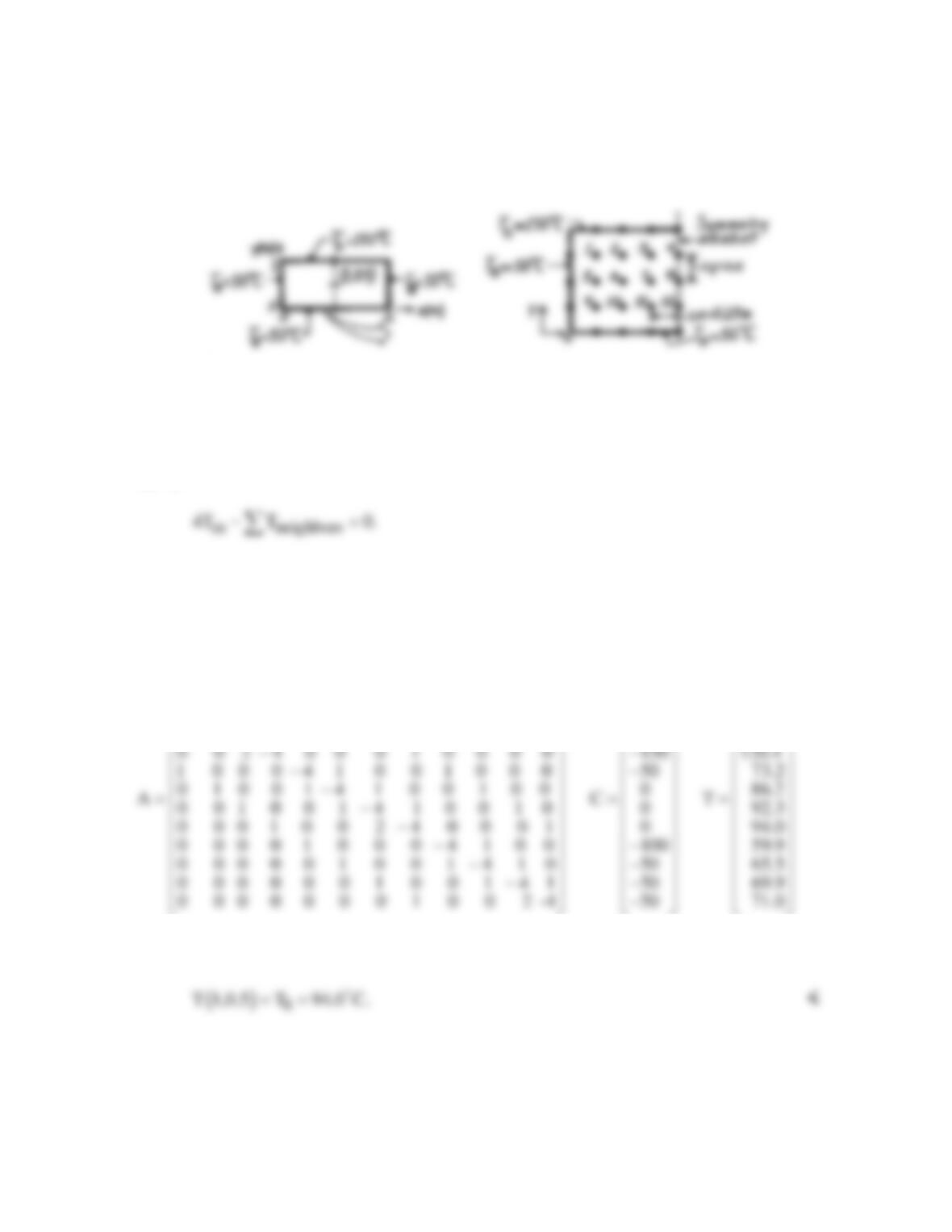
(b) Using the Finite-Difference Equations option from the Tools portion of the IHT menu, the following
two-dimensional temperature field was computed for the grid shown in schematic (b), where x and y are
in mm and the nodal temperatures are in °C. Nodes 2-54 are interior nodes, with those along the
symmetry adiabats characterized by Tm-1,n = Tm+1,n, while nodes 55-63 lie on a plane surface.
y\x
0
10
20
30
40
50
60
70
80
0
200
200
200
200
200
10
200
191
186.6
184.3
183.1
182.8
20
200
186.7
177.2
171.2
167.5
165.5
164.8
30
200
182.4
169.5
160.1
153.4
149.0
146.4
145.5
40
200
175.4
160.3
148.9
140.1
133.5
128.7
125.7
124.4
50
141.4
134.3
125.7
118.0
111.6
106.7
103.1
100.9
100.1
60
97.09
94.62
90.27
85.73
81.73
78.51
76.17
74.73
74.24
70
57.69
56.83
55.01
52.95
51.04
49.46
48.31
47.60
47.36
80
20
20
20
20
20
20
20
20
20
The foregoing results were computed for h = 107 W/m2⋅K (h → ∞) and T∞ = 20°C, which is tantamount
to prescribing an isothermal bottom surface at 20°C. Agreement between corresponding results for the
coarse and fine grids is surprisingly good (Ta = 135.7°C ↔ T23 = 140.1°C; Tb = 122.9°C ↔ T27 =
124.4°C). The heat rate is
NOTE TO INSTRUCTOR: To reduce computational effort, while achieving the same educational
objectives, the problem statement has been changed to allow for convection at the bottom, rather than the
top, surface.
PROBLEM 4.67
KNOWN: Rectangular plate subjected to uniform temperature boundaries.
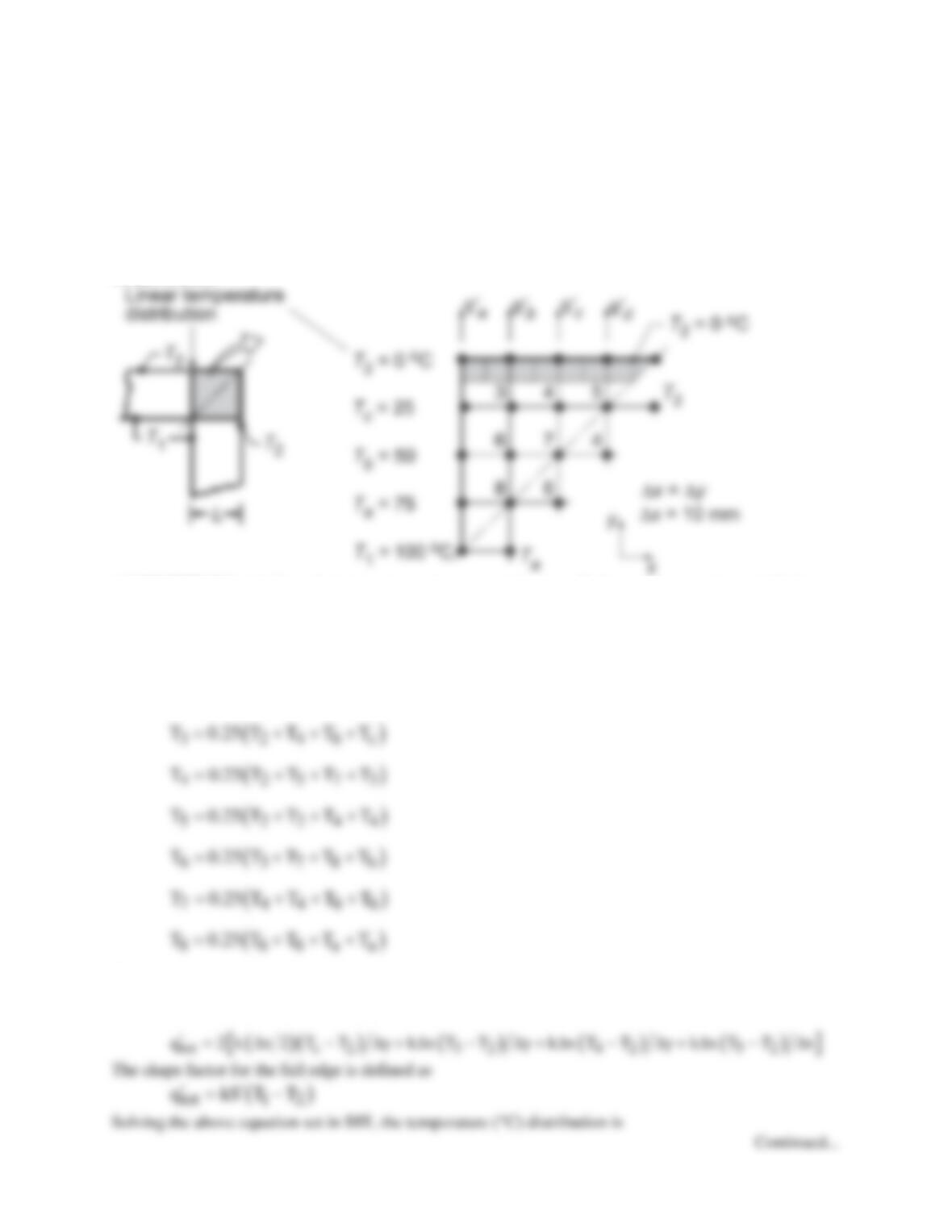
FIND: Temperature at the midpoint using a finite-difference method with space increment of 0.25m
SCHEMATIC:
ASSUMPTIONS: (1) Steady-state conditions, (2) Two-dimensional conduction, (3) Constant
properties.
ANALYSIS: For the nodal network above, 12 finite-difference equations must be written. It follows
that node 8 represents the midpoint of the rectangle. Since all nodes are interior nodes, Eq. 4.29 is
appropriate and is written in the form
For nodes on the symmetry adiabat, the neighboring nodes include two symmetrical nodes. Hence,
for Node 4, the neighbors are Tb, T8 and 2T3. Because of the simplicity of the finite–difference
equations, we may proceed directly to the matrices [A] and [C] – see Eq. 4.48 – and matrix inversion
can be used to find the nodal temperatures Tm.
4 1 0 0 1 0 0 0 0 0 0 0
1 4 1 0 0 1 0 0 0 0 0 0
0 1 4 1 0 0 1 0 0 0 0 0
−−−−−
200
150
150
−
−
−
96.5
112.9
118.9
The temperature at the midpoint (Node 8) is
COMMENTS: Using the exact analytical, solution – see Eq. 4.19 and Problem 4.2 – the midpoint
temperature is found to be 94.5°C. To improve the accuracy of the finite-difference method, it would
be necessary to decrease the nodal mesh size.
PROBLEM 4.68
KNOWN: Edge of adjoining walls (k = 1 W/m⋅K) represented by symmetrical element bounded by the
diagonal symmetry adiabat and a section of the wall thickness over which the temperature distribution is
assumed to be linear.
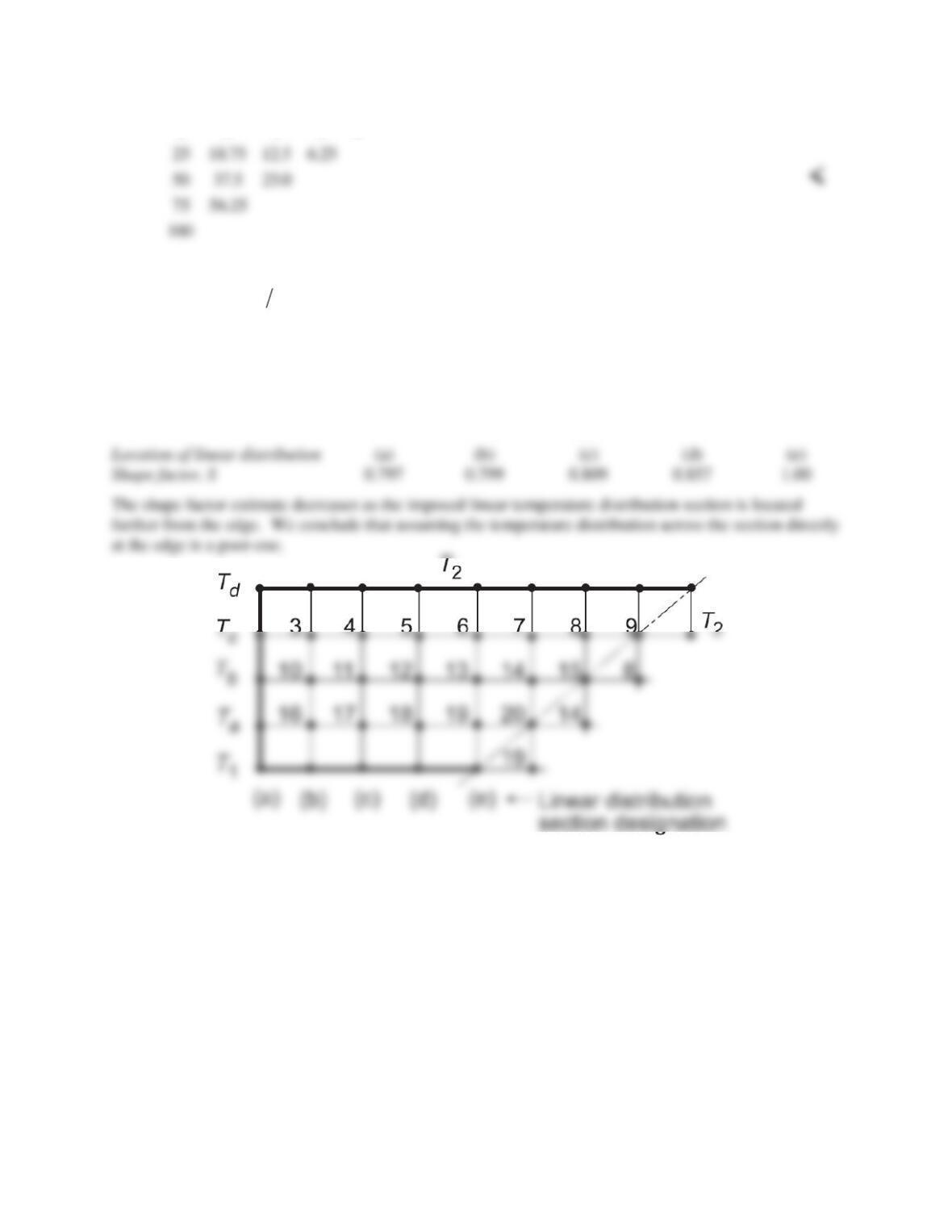
FIND: (a) Temperature distribution, heat rate and shape factor for the edge using the nodal network with
= ∆x = ∆y = 10 mm; compare shape factor result with that from Table 4.1; (b) Assess the validity of
assuming linear temperature distributions across sections at various distances from the edge.
SCHEMATIC:
ASSUMPTIONS: (1) Two–dimensional, steady-state conduction, (2) Constant properties, and (3) Linear
temperature distribution at specified locations across the section.
ANALYSIS: (a) Taking advantage of symmetry along the adiabat diagonal, all the nodes may be treated
as interior nodes. Across the left-hand boundary, the temperature distribution is specified as linear. The
finite–difference equations required to determine the temperature distribution, and hence the heat rate,
can be written by inspection.
The heat rate for both surfaces of the edge is
[ ]
tot a b c d
q 2q q q q
′ ′′′′
= +++
PROBLEM 4.68 (Cont.)
0 0 0 0 0
and the heat rate and shape factor are
tot
q 100 W m S 1
′= =
<
From Table 4.1, the edge shape factor is 0.54, considerably below our estimate from this coarse grid
analysis.
(b) The effect of the linear temperature distribution on the shape factor estimate can be explored using a
more extensive grid as shown below. The FDE analysis was performed with the linear distribution
imposed as the different sections a, b, c, d, e. Following the same approach as above, find
COMMENTS: The grid spacing for this analysis is quite coarse making the estimates in poor agreement
with the Table 4.1 result. However, the analysis does show the effect of positioning the linear
temperature distribution condition.
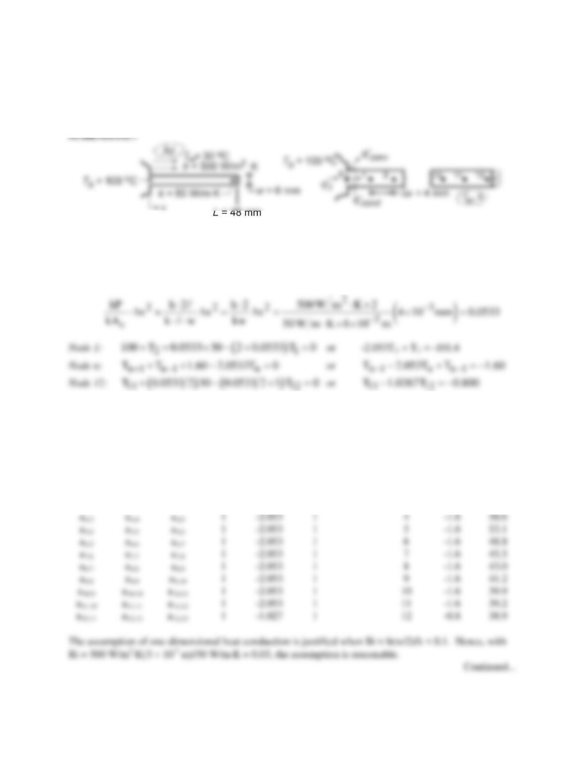
PROBLEM 4.69
KNOWN: Straight fin of uniform cross section with insulated end.
FIND: (a) Temperature distribution using finite-difference method and validity of assuming one-
dimensional heat transfer, (b) Fin heat transfer rate and comparison with analytical solution, Eq. 3.81, (c)
Effect of convection coefficient on fin temperature distribution and heat rate.
ASSUMPTIONS: (1) Steady-state conditions, (2) One-dimensional conduction in fin, (3) Constant
properties, (4) Uniform film coefficient.
ANALYSIS: (a) From the analysis of Problem 4.45, the finite-difference equations for the nodal
arrangement can be directly written. For the nodal spacing ∆x = 4 mm, there will be 12 nodes. With
>> w representing the distance normal to the page,
Using matrix notation, Eq. 4.48, where [A] [T] = [C], the A–matrix is tridiagonal and only the non-zero
terms are shown below. A matrix inversion routine was used to obtain [T].
Tridiagonal Matrix A
Column Matrices
Nonzero Terms
Values
Node
C
T
a1,1
a1,2
-2.053
1
1
-101.6
85.8
a2,1
a2,2
a2,3
1
-2.053
1
2
-1.6
74.5
a3,2
a3,3
a3,4
1
-2.053
1
3
-1.6
65.6
a4,3
a4,4
a4,5
1
-2.053
1
4
-1.6
58.6
a5,4
a5,5
a5,6
1
-2.053
1
5
-1.6
53.1
a6,5
a6,6
a6,7
1
-2.053
1
6
-1.6
48.8
a7,6
a7,7
a7,8
1
-2.053
1
7
-1.6
45.5
a8,7
a8,8
a8,9
1
-2.053
1
8
-1.6
43.0
a9,8
a9,9
1
-2.053
1
9
-1.6
41.2
1
-2.053
1
-1.6
39.9
1
-2.053
1
-1.6
39.2
1
-1.027
1
-0.8
38.9
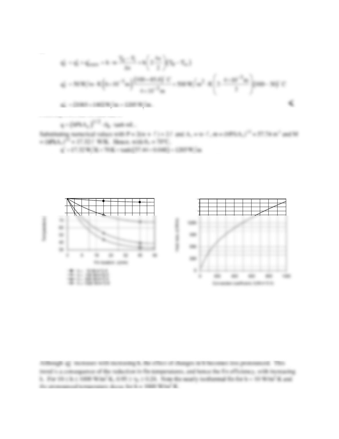
PROBLEM 4.69 (Cont.)
(b) The fin heat rate can be most easily found from an energy balance on the control volume about Node
0,
f
From Eq. 3.81, the fin heat rate is
and the finite-difference result agrees very well with the exact (analytical) solution.
(c) Using the IHT Finite-Difference Equations Tool Pad for 1D, SS conditions, the fin temperature
distribution and heat rate were computed for h = 10, 100, 500 and 1000 W/m2⋅K. Results are plotted as
follows.
80
90
100
1500
1800
The temperature distributions were obtained by first creating a Lookup Table consisting of 4 rows of
nodal temperatures corresponding to the 4 values of h and then using the LOOKUPVAL2 interpolating
function with the Explore feature of the IHT menu. Specifically, the function T_EVAL =
LOOKUPVAL2(t0467, h, x) was entered into the workspace, where t0467 is the file name given to the
Lookup Table. For each value of h, Explore was used to compute T(x), thereby generating 4 data sets
which were placed in the Browser and used to generate the plots. The variation of
q′
with h was simply
generated by using the Explore feature to solve the finite–difference model equations for values of h
incremented by 10 from 10 to 1000 W/m2⋅K.
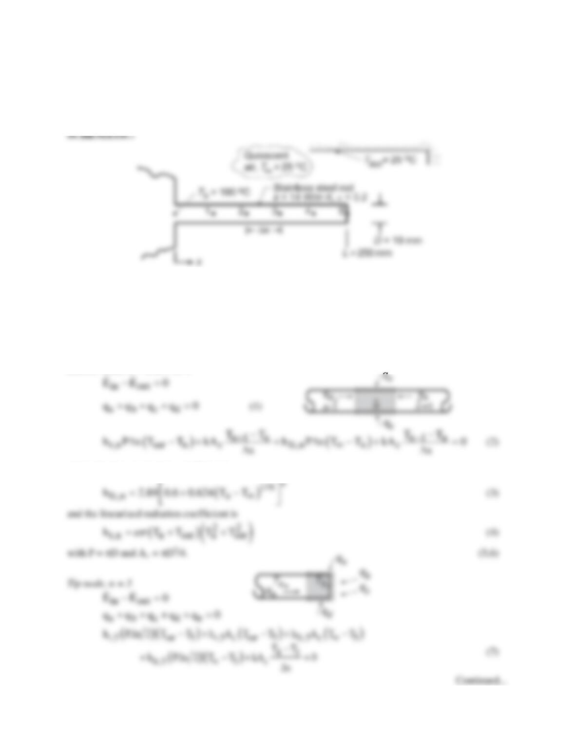
PROBLEM 4.70
KNOWN: Pin fin of 10 mm diameter and length 250 mm with base temperature of 100°C experiencing
radiation exchange with the surroundings and free convection with ambient air.
FIND: Temperature distribution using finite-difference method with five nodes. Fin heat rate and
relative contributions by convection and radiation.
ASSUMPTIONS: (1) Steady-state conditions, (2) One-dimensional conduction in fin, (3) Constant
properties, (4) Fin approximates small object in large enclosure, (5) Fin tip experiences convection and
radiation, (6) hfc = 2.89[0.6 + 0.624(T – T∞)1/6]2.
ANALYSIS: To apply the finite-difference method, define the 5-node system shown above where ∆x =
L/5. Perform energy balances on the nodes to obtain the finite-difference equations for the nodal
temperatures.
Interior node, n = 1, 2, 3 or 4
where the free convection coefficient is
PROBLEM 4.70 (Cont.)
Knowing the nodal temperatures, the heat rates are evaluated as:
Fin Heat Rate: Perform an energy balance around Node b.
x
∆
where hr,b and hfc,b are evaluated at Tb.
Convection Heat Rate: To determine the portion of the heat rate by convection from the fin surface, we
need to sum contributions from each node. Using the convection heat rate terms from the foregoing
energy balances, for, respectively, node b, nodes 1, 2, 3, 4 and node 5.
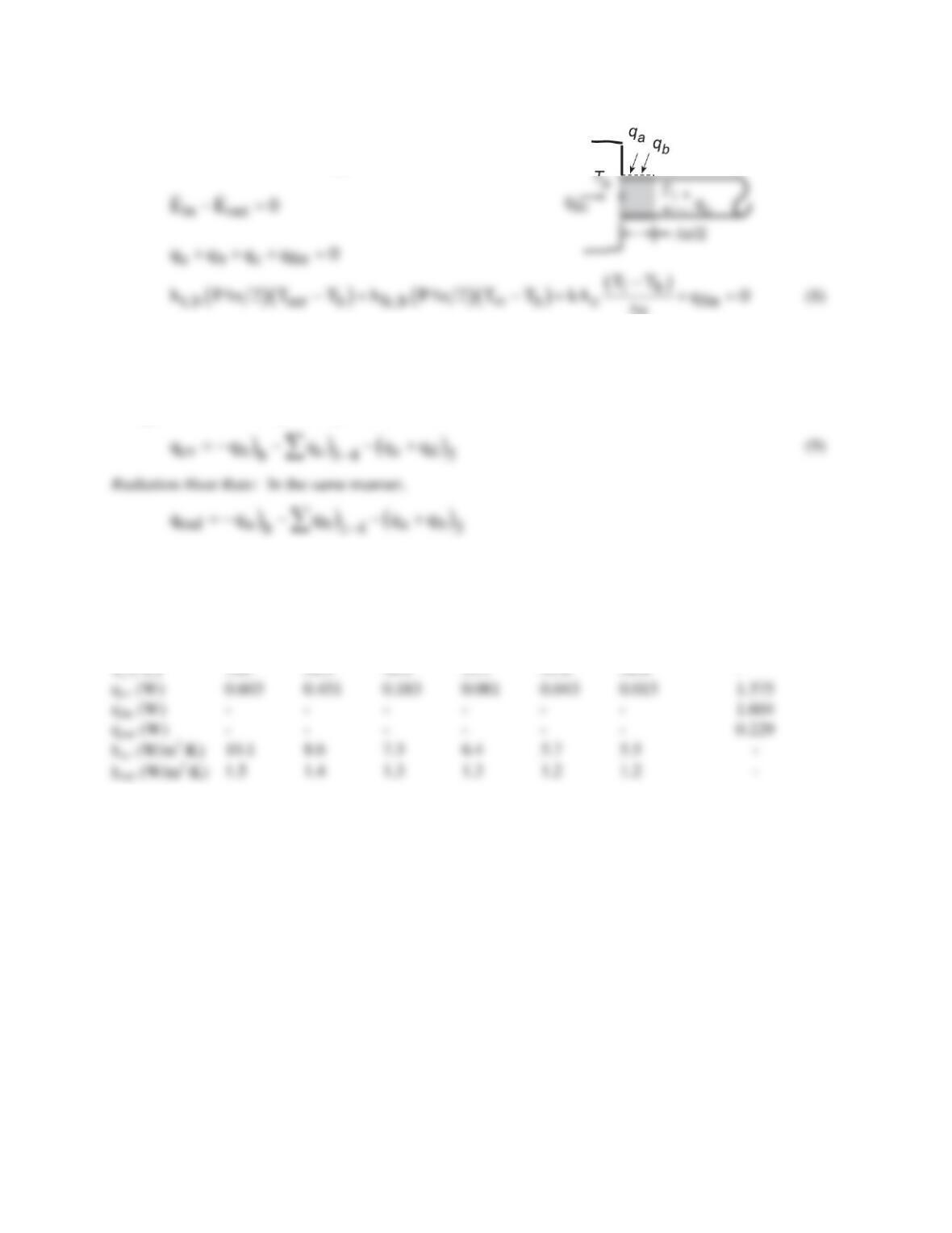
The above equations were entered into the IHT workspace and the set of equations solved for the nodal
temperatures and the heat rates. Summary of key results including the temperature distribution and heat
rates is shown below.
Node
b
1
2
3
4
5
Fin
<
COMMENTS: From the tabulated results, it is evident that free convection is the dominant node. Note
that the free convection coefficient varies almost by a factor of two over the length of the fin.
PROBLEM 4.71
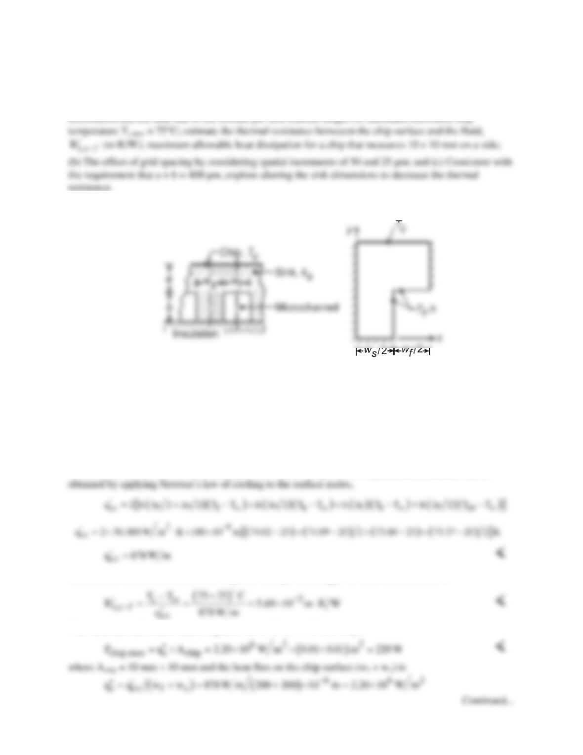
KNOWN: Heat sink for cooling computer chips fabricated from copper with microchannels passing
fluid with prescribed temperature and convection coefficient.
FIND: (a) Using a square nodal network with 100 µm spatial increment, determine the temperature
SCHEMATIC:
ASSUMPTIONS: (1) Steady-state, two–dimensional conduction, (2) Constant properties, and (3)
Convection coefficient is uniform over the microchannel surface and independent of the channel
dimensions and shape.
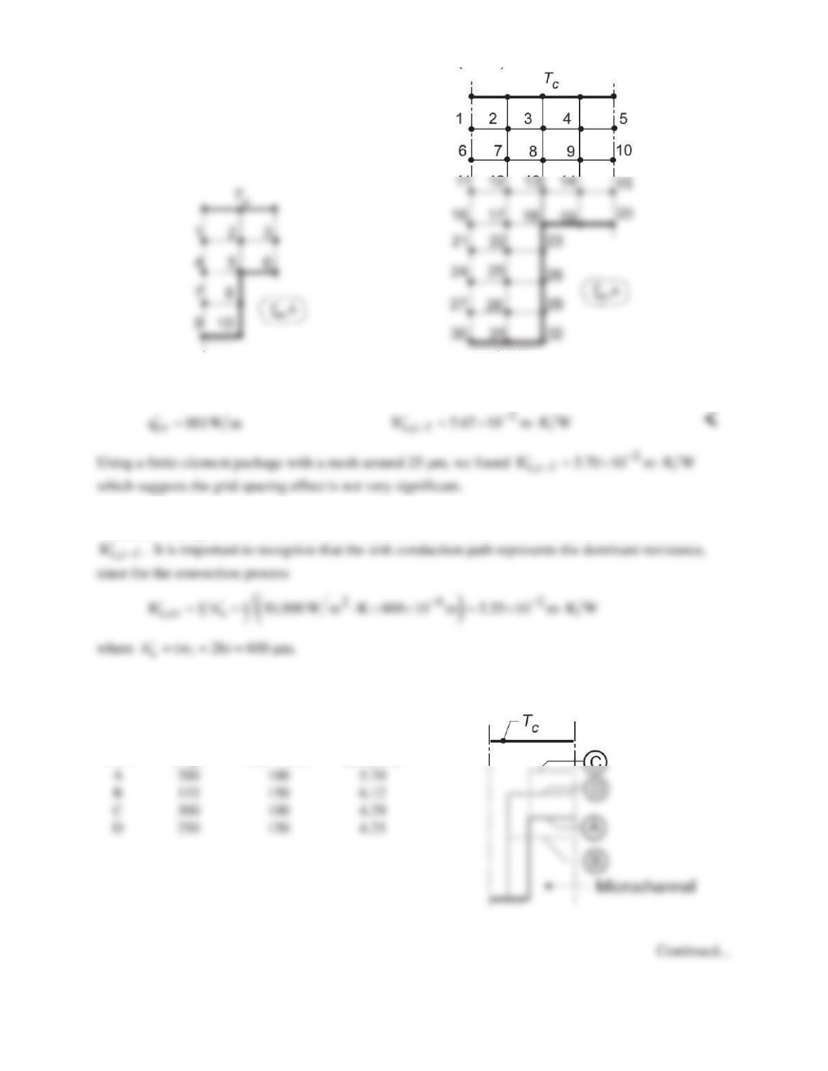
ANALYSIS: (a) The square nodal network with ∆x = ∆y = 100 µm is shown below. Considering
symmetry, the nodes 1, 2, 3, 4, 7, and 9 can be treated as interior nodes and their finite-difference
equations representing nodal energy balances can be written by inspection. Using the, IHT Finite–
Difference Equations Tool, appropriate FDEs for the nodes experiencing surface convection can be
obtained. The IHT code along with results is included in the Comments. Having the temperature
distribution, the heat rate to the coolant per unit channel length for two symmetrical elements can be
The thermal resistance between the chip and fluid per unit length for each microchannel is
The maximum allowable heat dissipation for a 10 mm × 10 mm chip is
PROBLEM 4.71 (Cont.)
(b) To investigate the effect of grid spacing, the analysis was repreated with a spatial increment of 50 µm
(32 nodes as shown above) with the following results
(c) Requring that the overall dimensions of the symmetrical element remain unchanged, we explored
what effect changes in the microchannel cross–section would have on the overall thermal resistance,
Using a finite–element package, the thermal resistances per unit length for three additional channel cross–
sections were determined and results summarized below.
Microchannel (µm)
t,c s
R−
′
× 10
2
Case
Height
Half–width
(m⋅K/W)