Section 9.4: Nonlinear Mechanical Systems 555
The coefficient matrix 12
81
A has real eigenvalues 13
and 25
of opposite
3
Problem 3
3.5
Problem 4
4. The linear system is 2
x
xy
, 43yxy
, because
32
sin cos 1
3! 2!
xy
xyx x
,
5. The critical points are of the form
0, n
, where n is an integer, so we substitute
x
u,
yvn
. Then
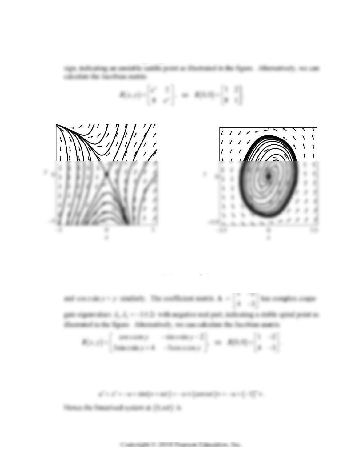
556 Chapter 9: Nonlinear Systems and Phenomena
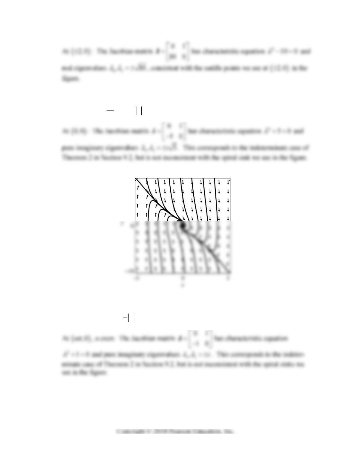
At
0, n
, n even: The Jacobian matrix 11
20
J has characteristic equation
220
and real eigenvalues 12
, 21
of opposite sign. Hence
0, n
is a
saddle point if n is even, as we see in the figure above.
Problem 5
4
Problem 6
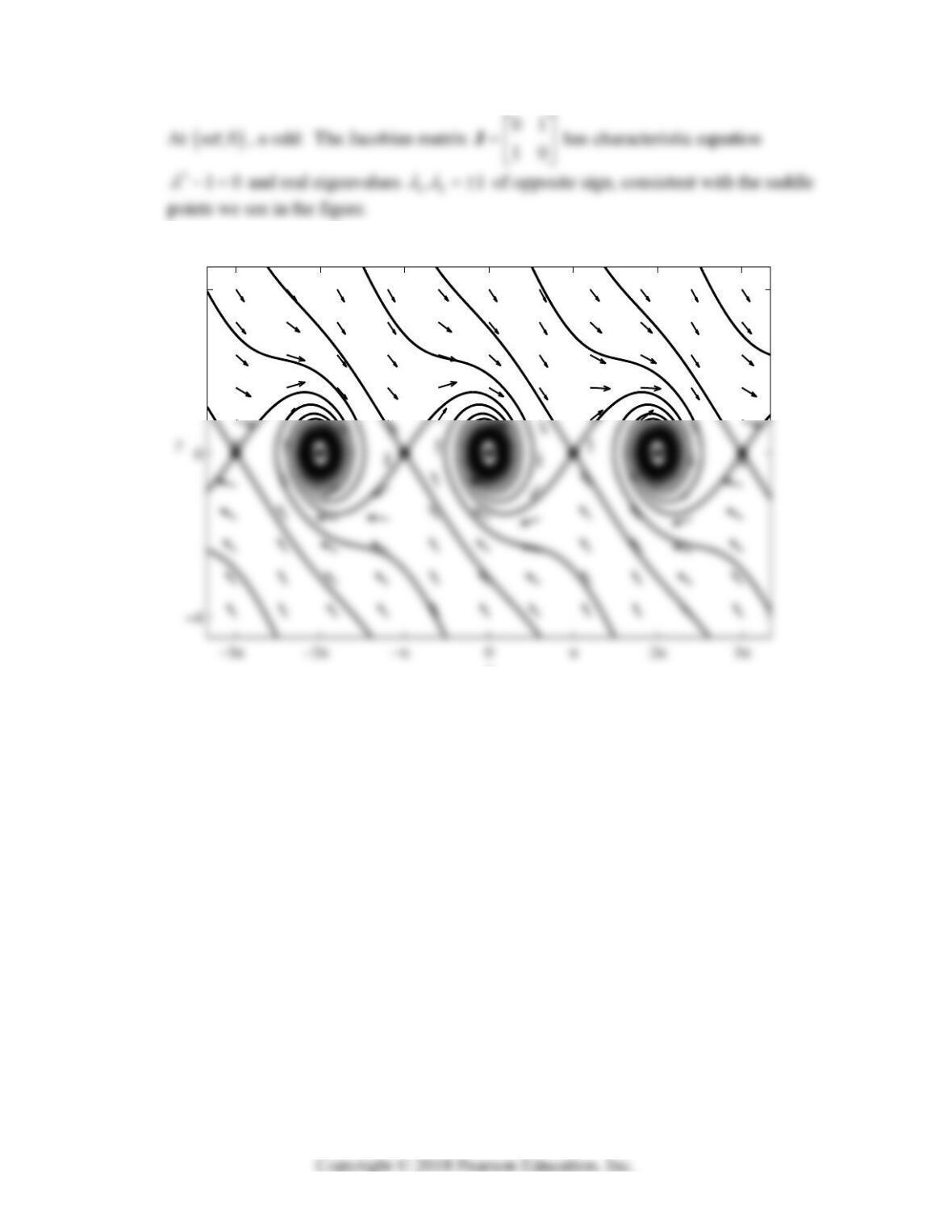
6. The critical points are of the form
,0n where n is an integer, so we substitute
x
un,
yv. Then
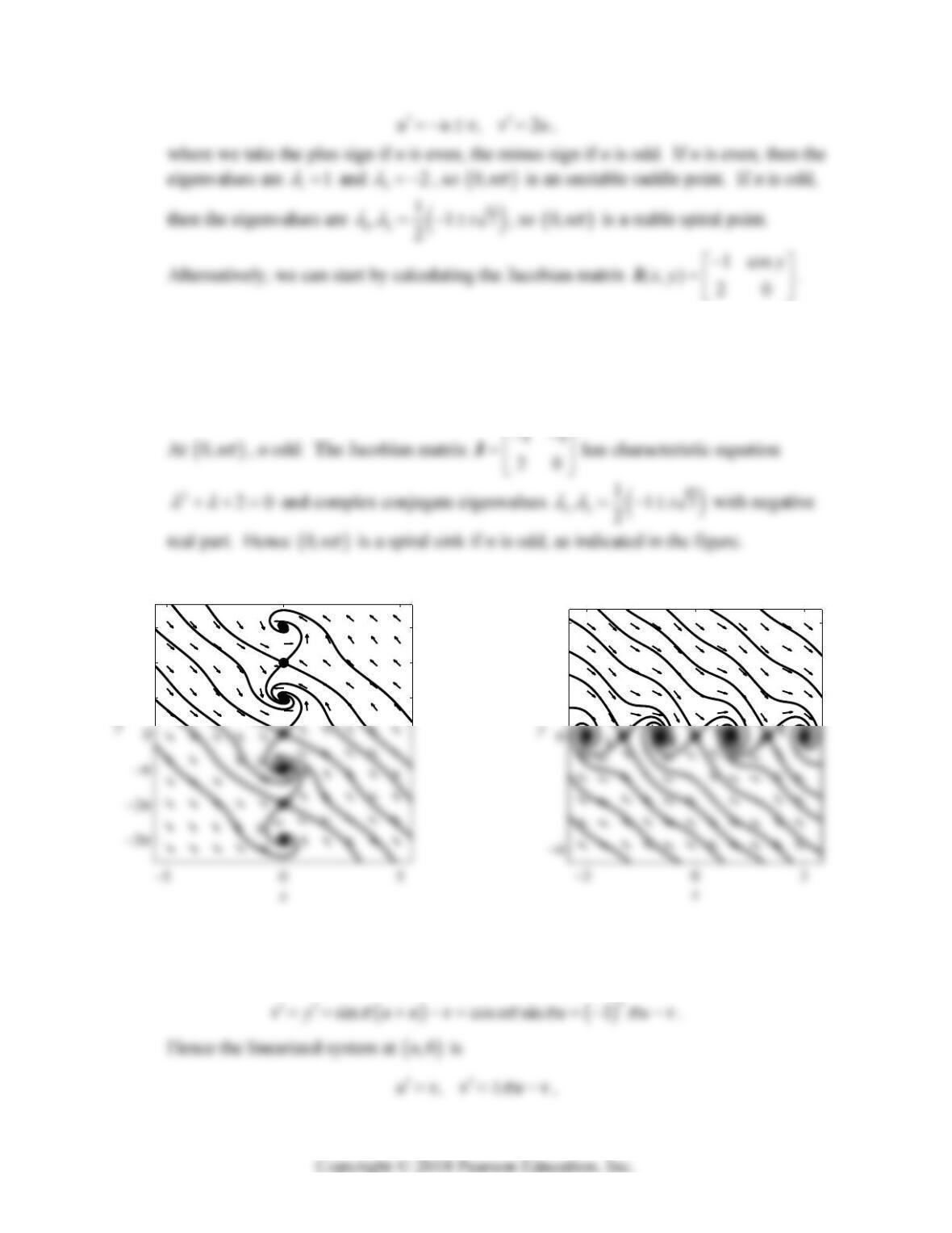
Section 9.4: Nonlinear Mechanical Systems 557
has complex conjugate roots with negative real part, so
,0n is a stable spiral point if n
is odd.
Alternatively, we can start by calculating the Jacobian matrix 01
(, ) cos 1
xy x
J.
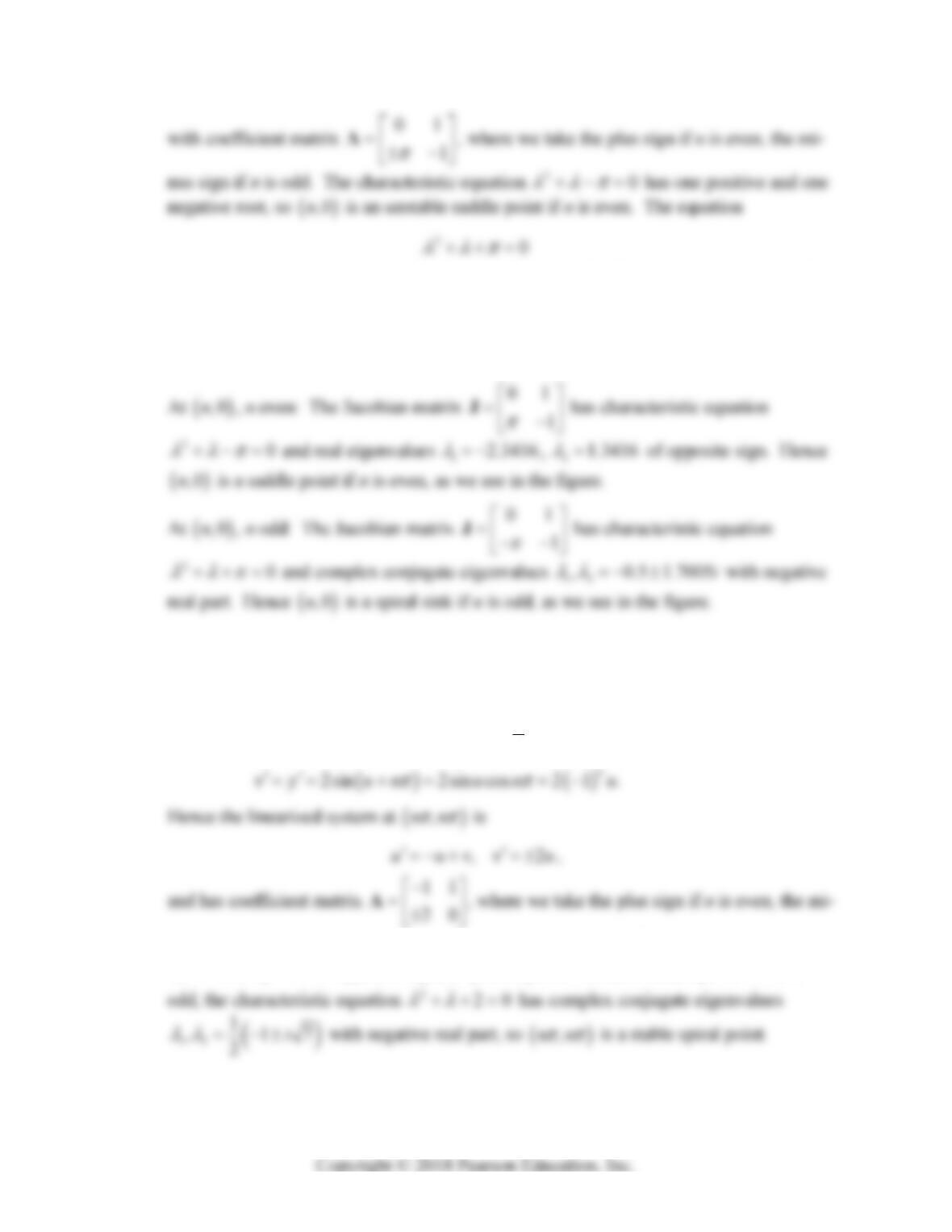
7. The critical points are of the form
,nn
, where n is an integer, so we substitute
x
un
, yvn
. Then
2
1
111 ,
2
uv
ux e uv uv uv
nus sign if n is odd. With n even, the characteristic equation 220
has real roots
11
and 22
of opposite sign, so
,nn
is an unstable saddle point. With n
558 Chapter 9: Nonlinear Systems and Phenomena
Alternatively, we can start by calculating the Jacobian matrix
,2cos 0
x
yxy
ee
xy x
J.
x
Problem 7
x
Problem 8
8. The critical points are of the form
,0n
where n is an integer, so we substitute
x
un
, yv. Then
3sin 3sin cos 3 1 ,
n
n
u x un v u n v uv
Section 9.4: Nonlinear Mechanical Systems 559
odd, then the characteristic equation 2550
has real roots
12
1
,121
2
with opposite signs, so
,0n
is an unstable saddle point.
As preparation for Problems 9–11, we first calculate the Jacobian matrix
2
01
(, ) cos
xy
x
c
J
of the damped pendulum system in (34) in the text. At the critical point
,0n
we have
9. If n is odd then the characteristic equation 22
0c
has real roots
10. If n is even, then the characteristic equation 22
0c
has roots
11. If n is even and 22
4c
, then the two eigenvalues
560 Chapter 9: Nonlinear Systems and Phenomena
Problems 12-16 call for us to find and classify the critical points of the first order-system
x
y
,
(, )
y
fxy
that corresponds to the given equation
,0xfxx
. After finding the critical
points
,0
x
where
,0 0fx , we first calculate the Jacobian matrix
,
x
yJ.
12.
2
01
,15 20 0
xy x
J.
13.
2
01
,15 20 2
xy x
J.
At
0, 0 : The Jacobian matrix 01
20 2
J has characteristic equation
Section 9.4: Nonlinear Mechanical Systems 561
14.
2
01
,86 0
xy x
J.
At
0, 0 : The Jacobian matrix 01
80
J has characteristic equation 280
and
15. 01
(, ) 240
xy x
J.
At
0, 0 : The Jacobian matrix 01
40
J has characteristic equation 240
and
16.
24
01
,415 5 0
xy xx
J.
At
0, 0 : The Jacobian matrix 01
40
J has characteristic equation 240
and
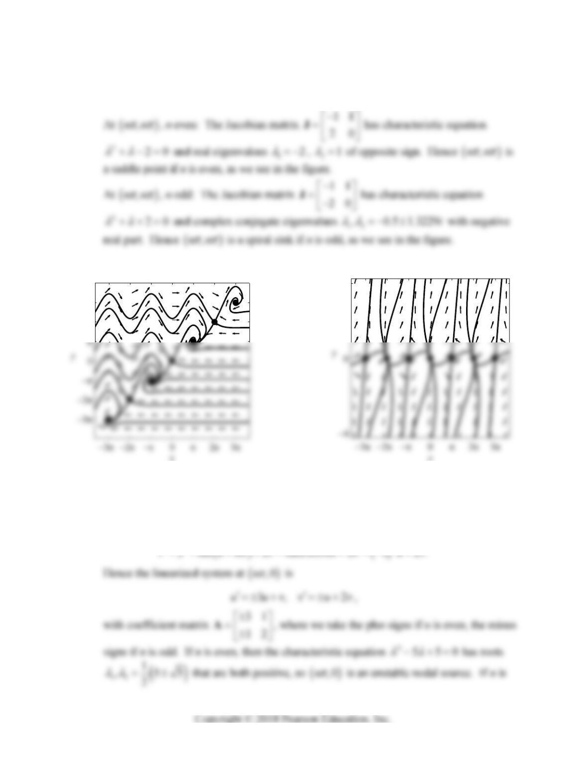
562 Chapter 9: Nonlinear Systems and Phenomena
17.
2
01
,15
52
4
xy x
J.
10
Problem 17
5
Problem 18
18.
2
01
,15
54
4
xy
x
y
J.
Section 9.4: Nonlinear Mechanical Systems 563
19.
2
01
,15
54
4
xy
x
y
J.
10
Problem 19
20.
01
,1
cos 2
xy
x
y
J.
564 Chapter 9: Nonlinear Systems and Phenomena
x
Problem 20
The statements of Problems 21–26 in the text include their answers and rather fully outline their
solutions, which therefore are omitted here.
565
CHAPTER 10
LAPLACE TRANSFORM METHODS
SECTION 10.1
LAPLACE TRANSFORMS AND INVERSE TRANSFORMS
The objectives of this section are especially clear cut. They include familiarity with the definition
of the Laplace transform L{f(t)} = F(s) that is given in Equation (1) in the textbook, the direct
application of this definition to calculate Laplace transforms of simple functions (as in Examples
1–3), and the use of known transforms (those listed in Figure 10.1.2) to find Laplace transforms
and inverse transforms (as in Examples 4–6). Perhaps students need to be told explicitly to
memorize the transforms that are listed in the short table that appears in Figure 10.1.2.
1. 0
}
{(,)
st
t e t dt u st du s dt
L
2. We substitute u = –st in the tabulated integral
22
22
uu
ue du e u u C
4. With a = –s and b = 1 the tabulated integral
22
cos sin
cos
au au abubbu
ebudue C
ab
566 Chapter 10: Laplace Transform Methods
5.
(1) (1)
11 1
22 2
00
2
sinh
11 1 1
21 1 1
tt sttt st st
t e e e e e dt e e dt
ss s
LL
7.
1
1
00
11
()
s
st st e
ft e dt e
ss
L
s
s
10.
1
1
222
0
0
11 11
() (1 )
s
st st te
ft te dt e sss ss s
L
11.
3/2 2 3/2 2
(3/ 2) 1 3
33
2
tt ssss
L
12.
5/2 3
7/2 4 7/2 2
(7 / 2) 3! 45 24
34 3 4 8
tt ssss
L
Section 10.1: Laplace Transforms and Inverse Transforms 567
16.
22 2
22
sin 2 cos 2 44 4
ss
tt
ss s
L
17.
2
2
111
cos 2 1+cos4
2216
s
tt
ss
LL
20. Integrating by parts with u = t, dv = e–(s–1)tdt, we get
(1)
00
(1)
2
0
0
111
.
11 1(1)
tstt st
st
st t
te e te dt te dt
te eedt t
ss s s
L
L
21. Integration by parts with u = t and dv = e–stcos 2t dt yields
22.
2
2
111
sinh 3 cosh 6 1
2236
s
tt
ss
LL
23. 11 3
44
3161
22
t
ss
LL
568 Chapter 10: Laplace Transform Methods
26. 15
1
5
t
e
s
L
29. 111
222
53 5 3 5
3sin33cos3
93 9 93
ss
tt
sss
LLL
32.
3
1
3
22(3)2()
s
eut u t
s
L [See Example 8 in the textbook.]
35. Using the given tabulated integral with a = –s and b = k, we find that
Section 10.1: Laplace Transforms and Inverse Transforms 569
37. ()
f
t = 1 – ua(t) = 1 – u(t – a) so
38. ()()(),
f
tutautbso
39. Use of the geometric series gives
11
sse
se
40. Use of the geometric series gives
41. By checking values at sample points, you can verify that ( ) 2 ( )1gt f t in terms of
the square wave function ( )
f
t of Problem 40. Hence
570 Chapter 10: Laplace Transform Methods
1 sinh( / 2) 1 tanh .
cosh( / 2) 2
ss
ss s
42. Let’s refer to ( 1, ]nn as an odd interval if the integer n is odd, and even interval if n
is even. Then our function ( )ht has the value a on odd intervals, the value b on even
intervals. Now the unit step function ( )
f
t of Problem 40 has the value 1 on odd
SECTION 10.2
TRANSFORMATION OF INITIAL VALUE PROBLEMS
The focus of this section is on the use of transforms of derivatives (Theorem 1) to solve initial
value problems (as in Examples 1 and 2). Transforms of integrals (Theorem 2) appear less
frequently in practice, and the extension of Theorem 1 at the end of Section 10.2 may be
considered entirely optional (except perhaps for electrical engineering students).
In Problems 1–10 we give first the transformed differential equation, then the transform X(s) of
the solution, and finally the inverse transform x(t) of X(s).
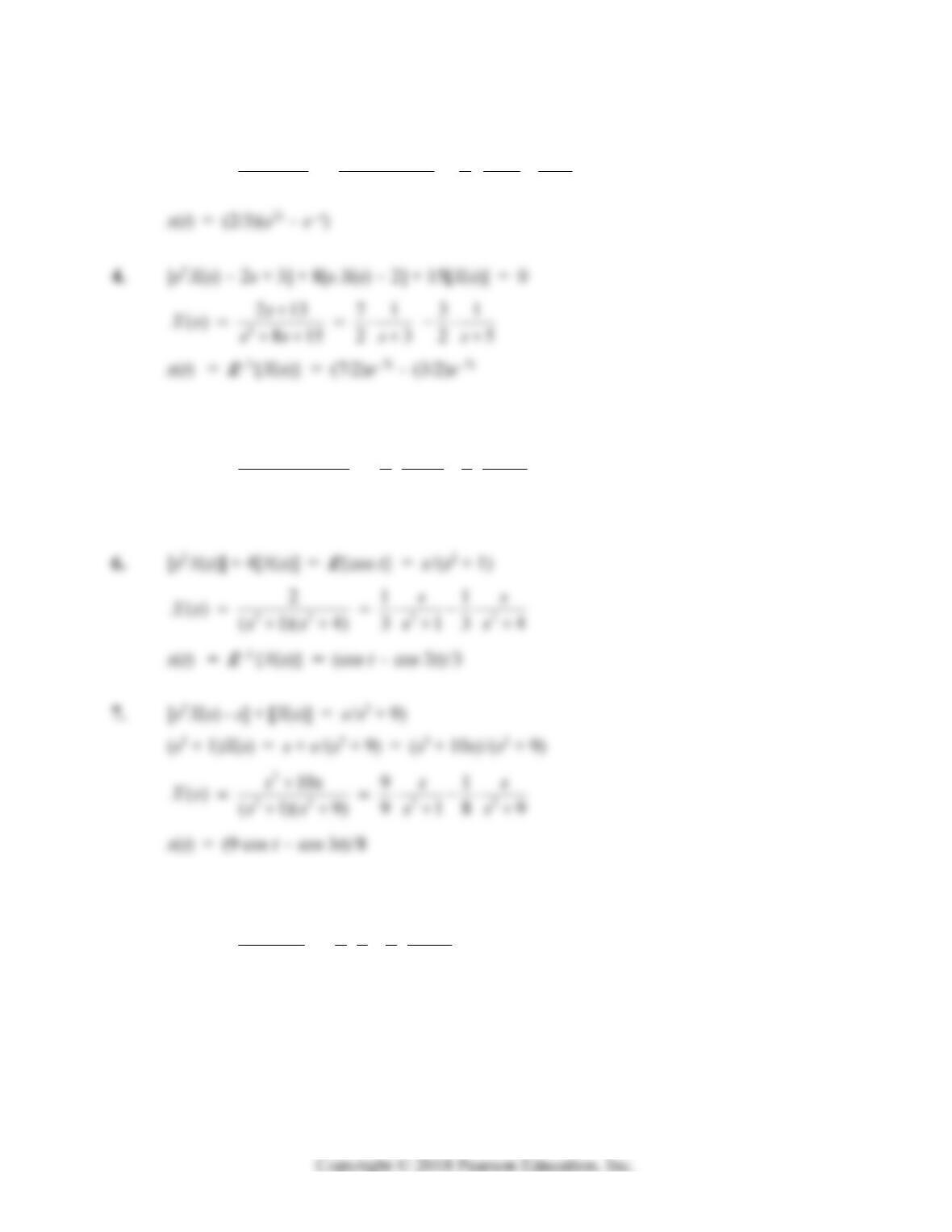
1. [s2X(s) – 5s] + 4{X(s)} = 0
Section 10.2: Transformation of Initial Value Problems 571
3. [s2X(s) – 2] – [sX(s)] – 2[X(s)] = 0
2
22211
() 2(2)(1)3 2 1
Xs ss s s s s
5. [s2X(s)] + [X(s)] = 2/(s2 + 4)
22 2 2
22112
() (1)(4)3 13 4
Xs ss s s
x(t) = (2 sin t – sin 2t)/3
8. [s2X(s)] + 9[X(s)] = L{1} = 1/s
22
1111
() (9)9 9 9
s
Xs ss s s
x(t) = L–1{X(s)} = (1 – cos 3t)/9
572 Chapter 10: Laplace Transform Methods
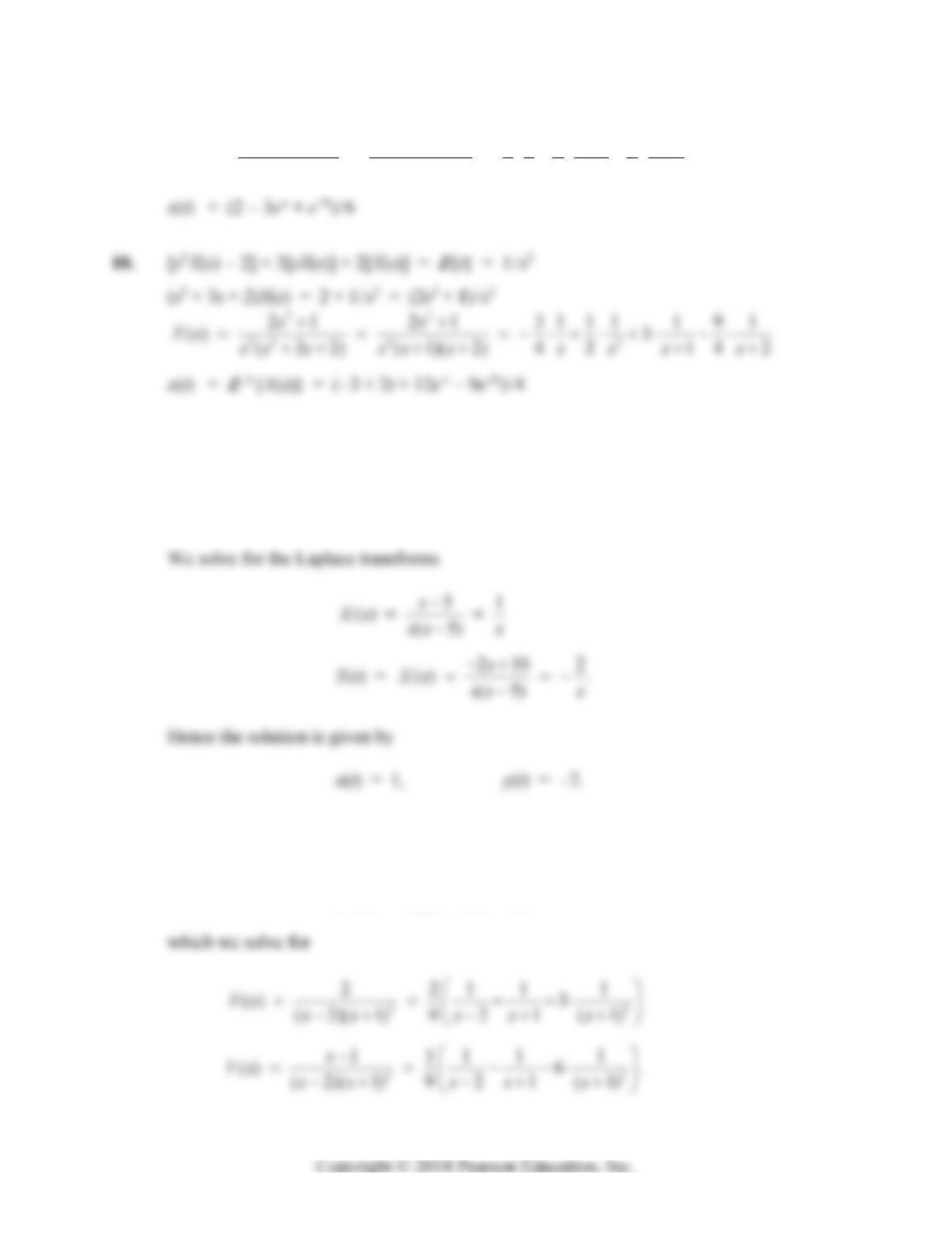
9. s2X(s) + 4sX(s) + 3X(s) = 1/s
2
11111111
() ( 4 3) ( 1)( 3) 3 2 1 6 3
Xs ss s ss s s s s
11. The transformed equations are
sX(s) – 1 = 2X(s) + Y(s)
sY(s) + 2 = 6X(s) + 3Y(s).
12. The transformed equations are
s X(s) = X(s) + 2Y(s)
s Y(s) = X(s) + 1/(s + 1),
Section 10.2: Transformation of Initial Value Problems 573
13. The transformed equations are
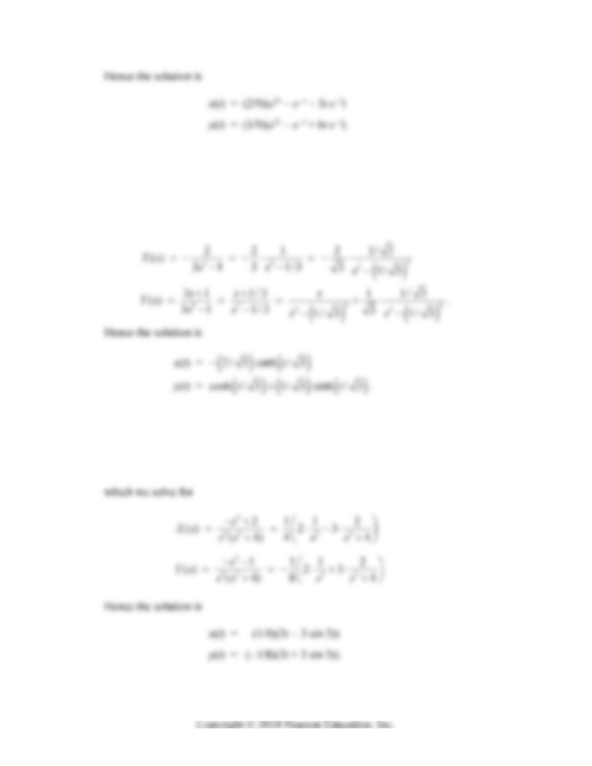
sX(s) + 2[sY(s) – 1] + X(s) = 0
sX(s) – [sY(s) – 1] + Y(s) = 0,
which we solve for the transforms
14. The transformed equations are
s2X(s) + 1 + 2X(s) + 4Y(s) = 0
s2Y(s) + 1 + X(s) + 2Y(s) = 0,
574 Chapter 10: Laplace Transform Methods
15. The transformed equations are
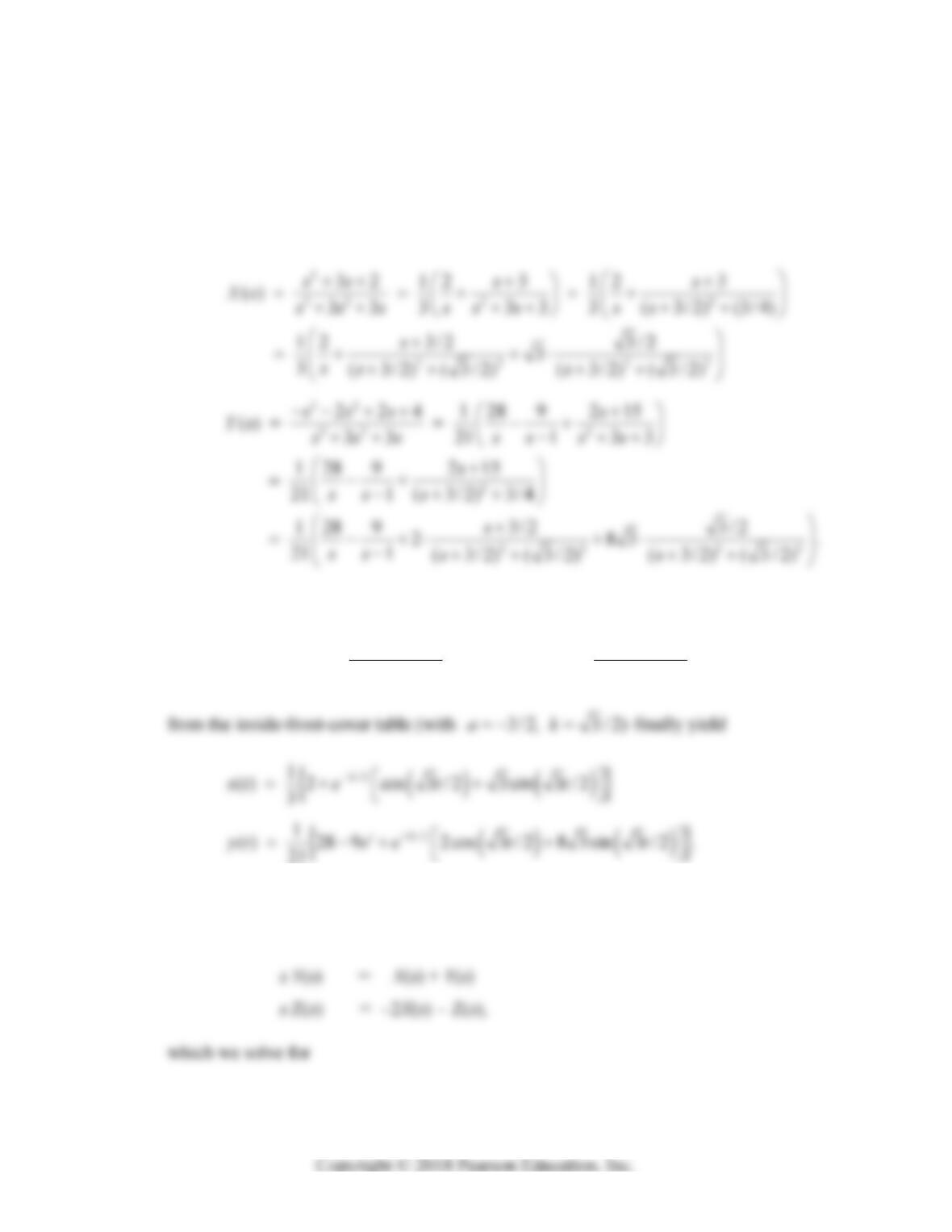
[s2X – s] + [sX – 1] + [sY – 1] + 2X – Y = 0
[s2Y – s] + [sX – 1] + [sY – 1] + 4X – 2Y = 0,
which we solve for
Here we’ve used some fairly heavy-duty partial fractions (Section 10.3). The transforms
22 22
cos , sin
() ()
at at
sa k
ekt ekt
sa k sa k
LL
16. The transformed equations are
s X(s) – 1 = X(s) + Z(s)