Section 9.2: Linear and Almost Linear Systems 535
3
x
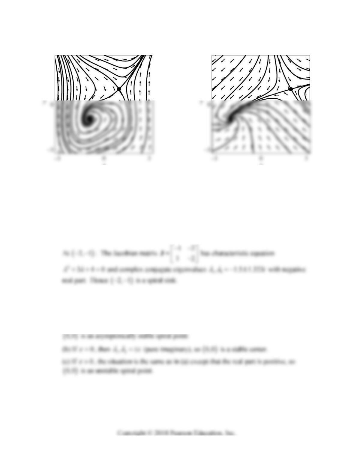
Problem 31
3
x
Problem 32
32. 12
y
x
J
At
2,1 : The Jacobian matrix 12
12
J has characteristic equation 240
and real eigenvalues 12.56
, 21.56
with different signs. Hence
2,1 is a sad-
dle point.
33. The characteristic equation of the given linear system is
210
, with character-
istic roots 12
,i
.
(a) So if
0
, then 12
,
are complex conjugates with negative real part, and hence
536 Chapter 9: Nonlinear Systems and Phenomena
34. The characteristic equation of the given linear system is
2
10e
.
(a) If 0
, then 12
,1i
. Thus the characteristic roots are complex conju-
35. (a) If 0h, then we have the familiar system
x
y
, yx
with circular trajectories
about the origin, which is therefore a center.
(b) The change to polar coordinates as in Example 5 of Section 9.1 is routine, yielding
36. (a) Again, the change of variables is essentially the same as in Example 5 of Section 9.1.
(b) If 2
a
then the equation
22
rrar
integrates to give the equation
22
22
ln
ln
2
ar
r
tC aa
,
which (after exponentiating) we readily solve for
Section 9.2: Linear and Almost Linear Systems 537
37. The substitution
y
vx in the homogeneous first-order equation
y
Separating the variables and integrating by partial fractions, we get
2
11 21
11
vdx
dv
vv v v x
,
or
x
x
x
x
38. The roots of the characteristic equation 20TD
are given by
2
12
4
,2
TT D
.
We examine the various possibilities individually.
538 Chapter 9: Nonlinear Systems and Phenomena
If the point
,TD lies on the positive D-axis, so 0T but 0D, then 12
iD
,
pure imaginary, so we have a stable center.
SECTION 9.3
ECOLOGICAL MODELS:
PREDATORS AND COMPETITORS
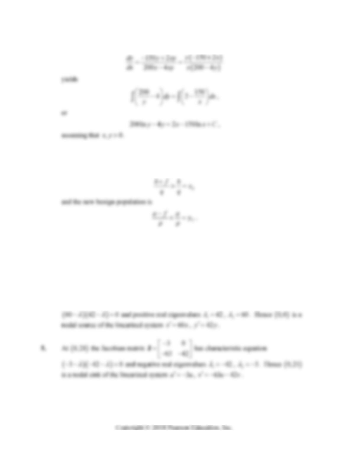
1. 200 4 4
2 150 2
yx
y
x
J
At
0, 0 : The Jacobian matrix 200 0
0 150
J has characteristic equation
5
x
Problem 1a
5
u
Problem 1b
Section 9.3: Ecological Applications: Predators and Competitors 539
2. Upon separation of variables, the equation
y
y
3. The effect of using the insecticide is to replace b by bf and a by af in the preda-
tor-prey equations, while leaving p and q unchanged. Hence the new harmful population
is
x
y
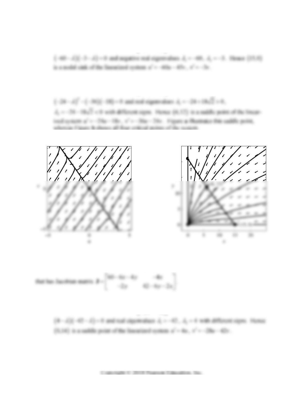
Problems 4–7 deal with the competition system
22
60 4 3 , 42 2 3
x
xx xyy yy xy
,
that has Jacobian matrix 60 8 3 3
34243
xy x
y
yx
J.
4. At
0, 0 the Jacobian matrix 60 0
042
J has characteristic equation
y
540 Chapter 9: Nonlinear Systems and Phenomena
6. At
15, 0 the Jacobian matrix 60 45
03
J has characteristic equation
7. At
6,12 the Jacobian matrix 24 18
36 24
J has characteristic equation
5
Problem 7a
15
20
(0, 21)
Problem 7b
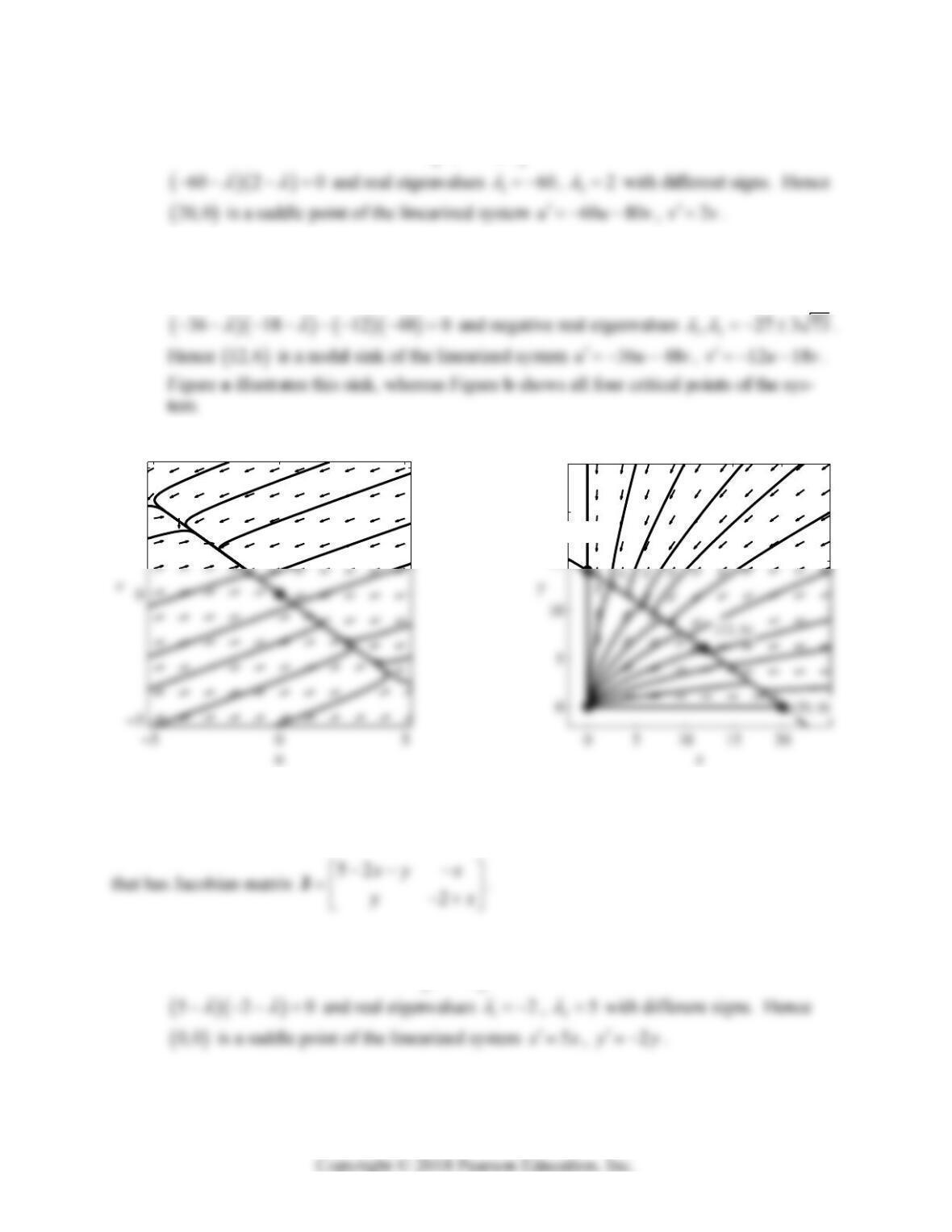
Problems 8–10 deal with the competition system
22
60 3 4 , 42 3 2
x
xx xyy yy xy
8. At
0,14 the Jacobian matrix 40
28 42
J has characteristic equation
Section 9.3: Ecological Applications: Predators and Competitors 541
9. At
20,0 the Jacobian matrix 60 80
02
J has characteristic equation
10. At
12,6 the Jacobian matrix 36 48
12 18
J has characteristic equation
5
Problem 10a
15
20
(0, 14)
Problem 10b
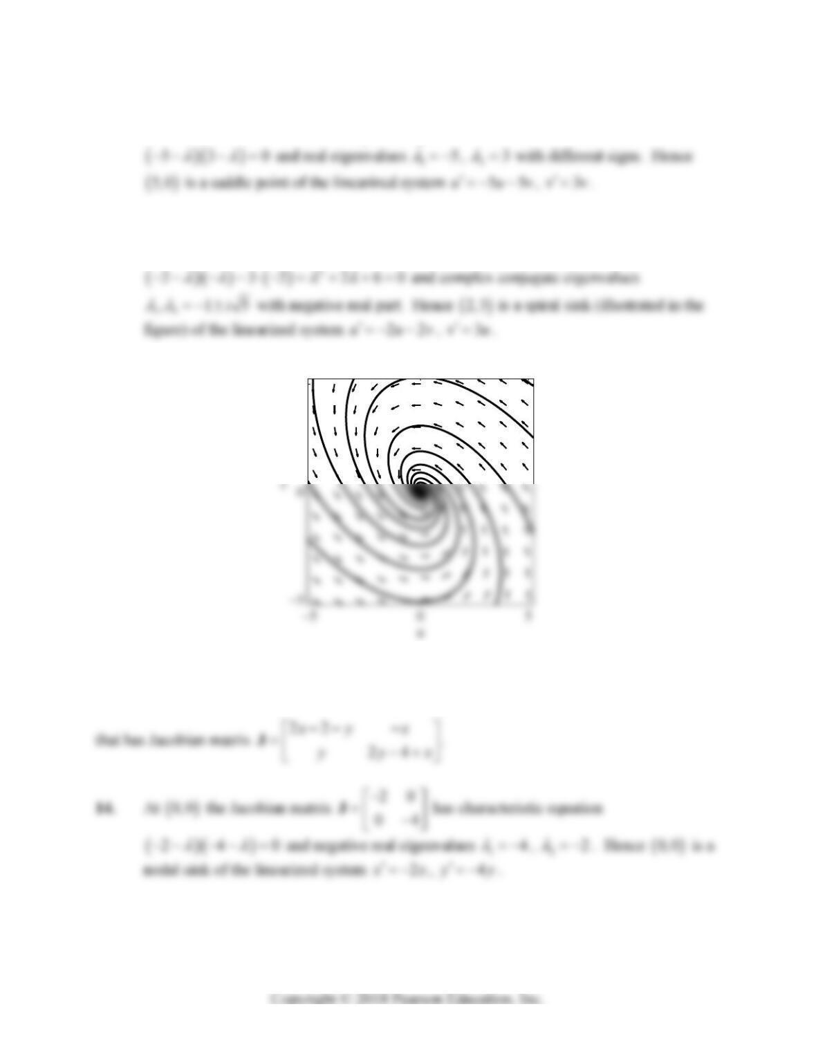
Problems 11–13 deal with the predator-prey system
2
5,2
x
x x xy y y xy
x
11. At (0,0) the Jacobian matrix 50
02
J has characteristic equation
542 Chapter 9: Nonlinear Systems and Phenomena
12. At
5, 0 the Jacobian matrix 55
03
J has characteristic equation
13. At
2,3 the Jacobian matrix 22
30
J has characteristic equation
5
Problem 13
Problems 14–17 deal with the predator-prey system
22
2, 4
x
xxxyyyyxy
Section 9.3: Ecological Applications: Predators and Competitors 543
15. At
0, 4 the Jacobian matrix 60
44
J has characteristic equation
16. At
2,0 the Jacobian matrix 22
02
J has characteristic equation
220
and real eigenvalues 12
, 22
with different signs. Hence
2,0 is a saddle point of the linearized system 22uuv
, 2vv
.
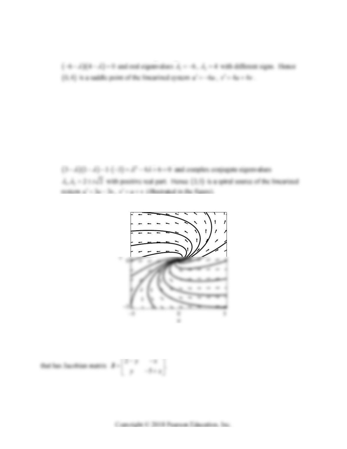
17. At
3,1 the Jacobian matrix 33
11
J has characteristic equation
system 33uuv
5
Problem 17
Problems 18 and 19 deal with the predator-prey system
2, 5
x
xxy y yxy
544 Chapter 9: Nonlinear Systems and Phenomena
18. At
0, 0 the Jacobian matrix 20
05
J has characteristic equation
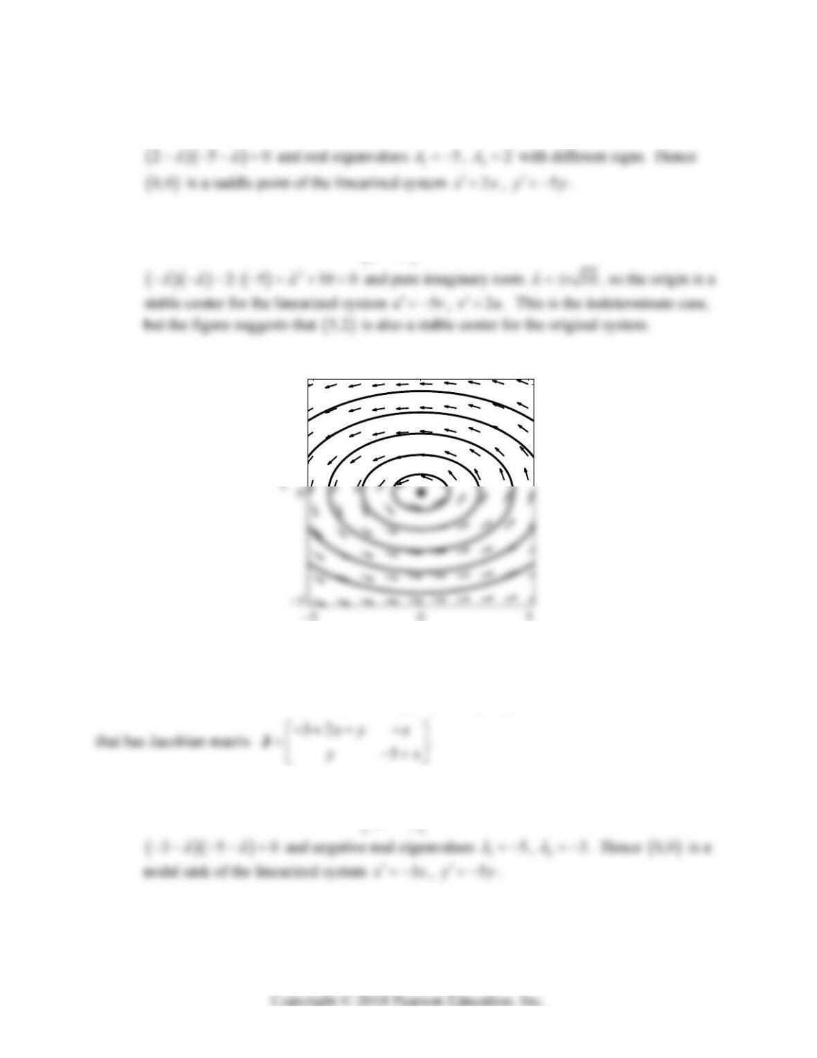
19. At
5, 2 the Jacobian matrix 05
20
J has characteristic equation
5
u
Problem 19
Problems 20–22 deal with the predator-prey system
2
3,5
x
x x xy y y xy
20. At (0,0) the Jacobian matrix 30
05
J has characteristic equation
Section 9.3: Ecological Applications: Predators and Competitors 545
21. At (3,0) the Jacobian matrix 33
02
J has characteristic equation
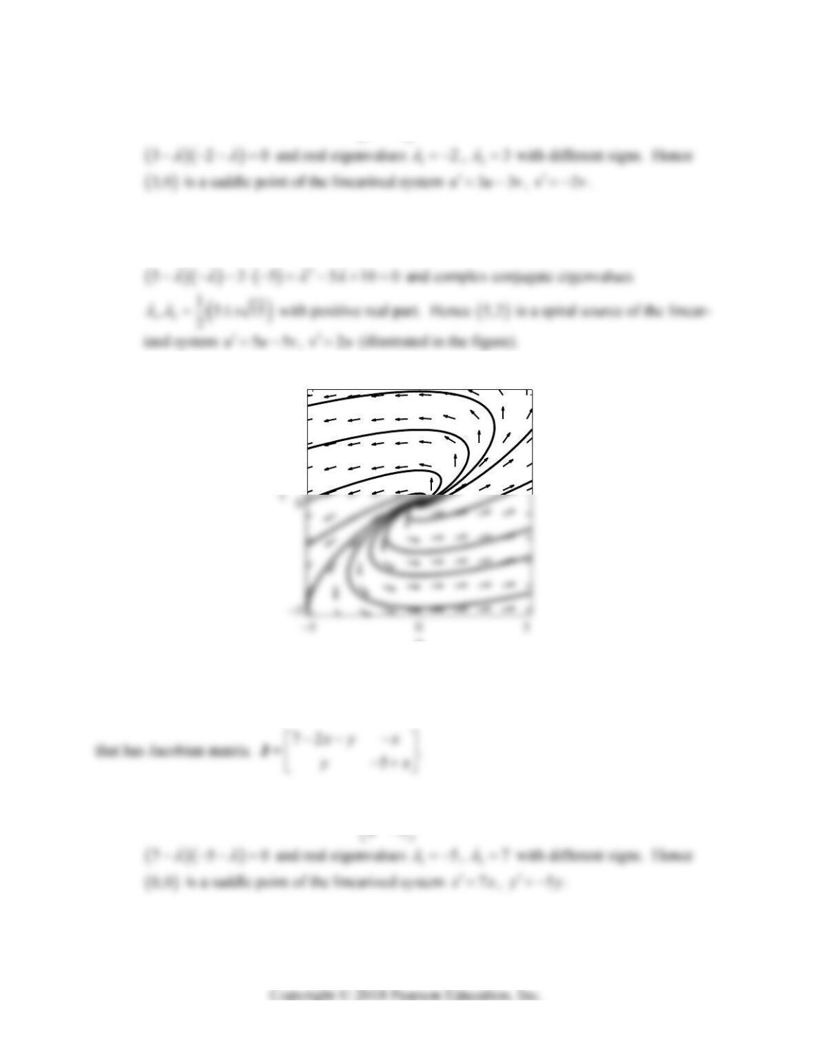
22. At
5, 2 the Jacobian matrix 55
20
J has characteristic equation
5
u
Problem 22
Problems 23–25 deal with the predator-prey system
2
7,5
x
x x xy y y xy
23. At (0,0) the Jacobian matrix 70
J has characteristic equation
546 Chapter 9: Nonlinear Systems and Phenomena
24. At (7,0) the Jacobian matrix 77
02
J has characteristic equation
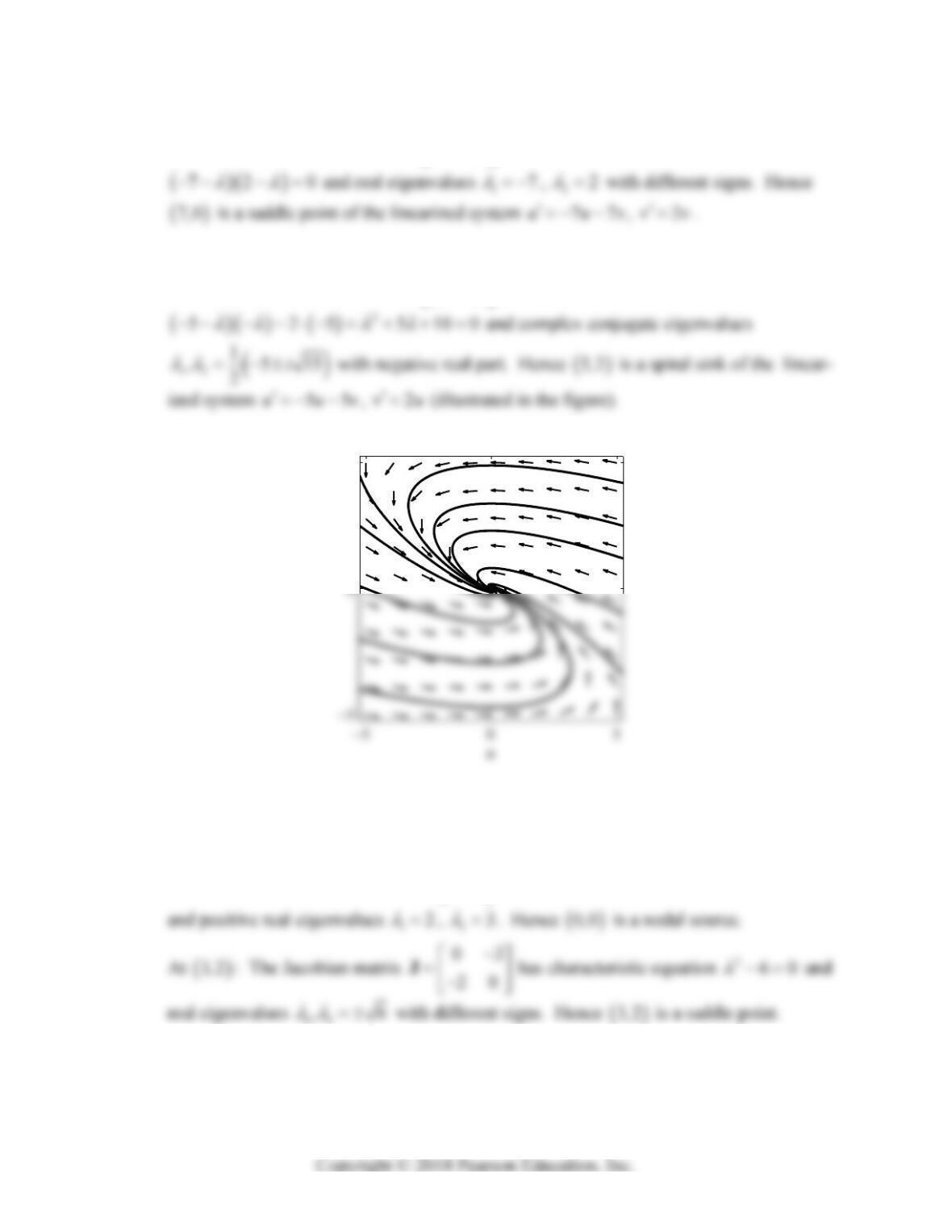
25. At
5, 2 the Jacobian matrix 55
20
J has characteristic equation
5
v
Problem 25
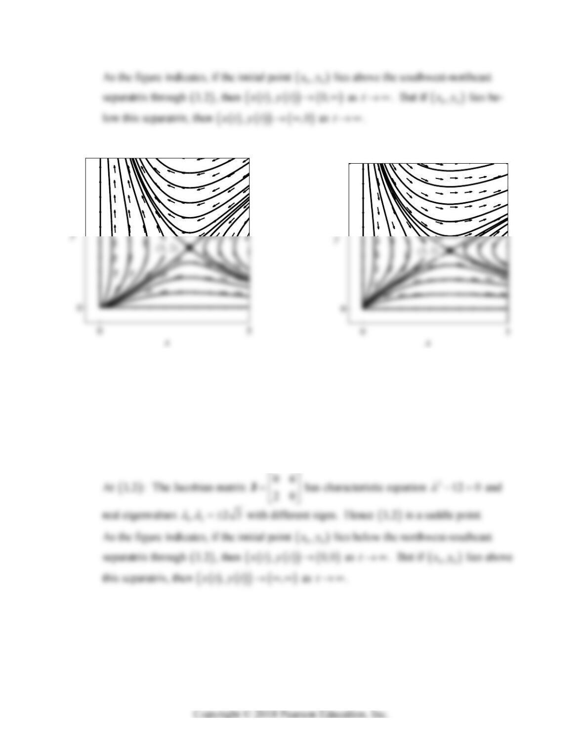
26. 2
3
y
x
y
x
J
At
0, 0 : The Jacobian matrix 20
03
J has characteristic equation 2560
Section 9.3: Ecological Applications: Predators and Competitors 547
5
Problem 26
5
Problem 27
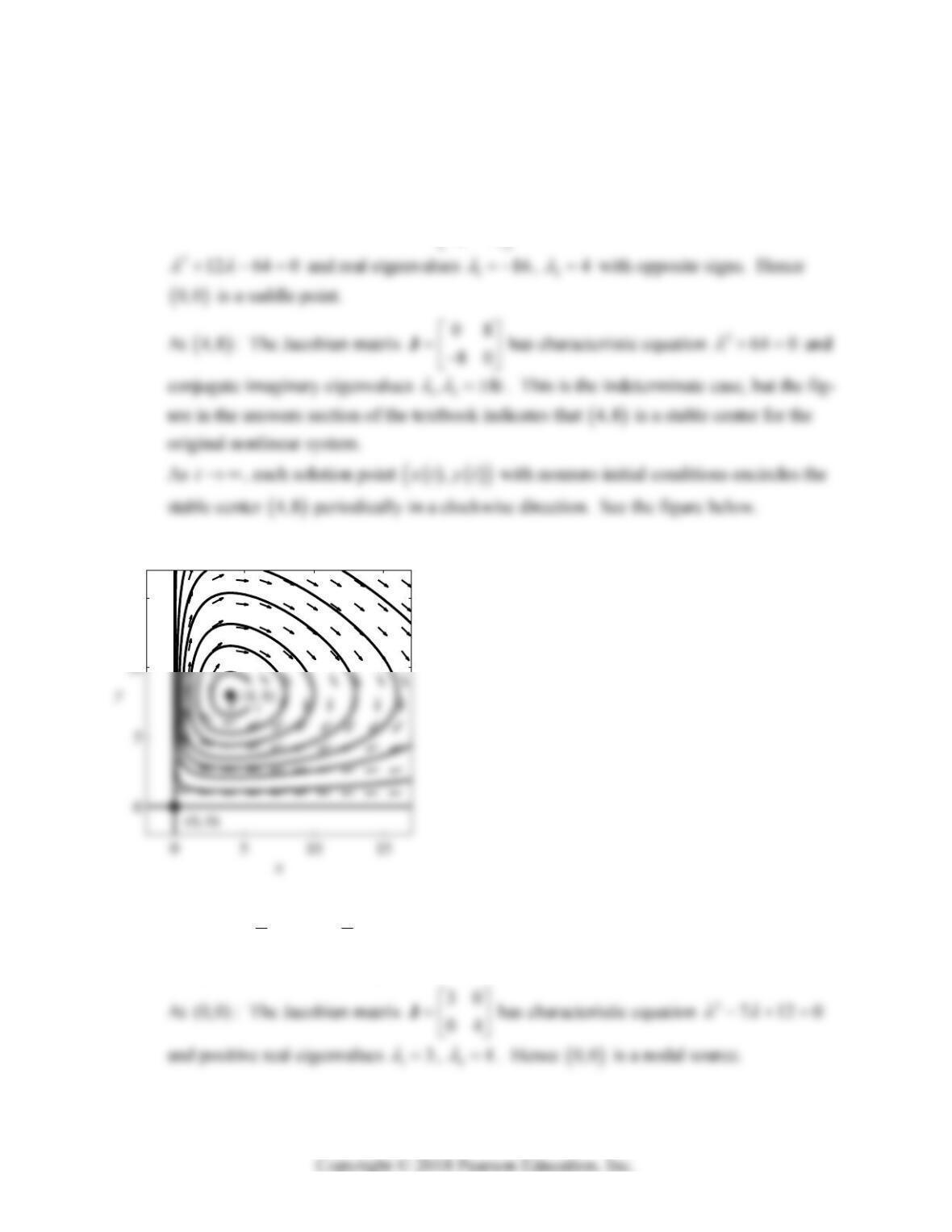
27. 242
3
y
x
yx
J
At
0, 0 : The Jacobian matrix 40
03
J has characteristic equation
27120
and negative real eigenvalues 14
, 23
. Hence
0, 0 is a nod-
al sink.
548 Chapter 9: Nonlinear Systems and Phenomena
28. 2162
4
y
x
y
x
J
At (0,0) : The Jacobian matrix 16 0
04
J has characteristic equation
15
Problem 28
29.
11
23
22
242
x
yx
yx
J
Section 9.3: Ecological Applications: Predators and Competitors 549
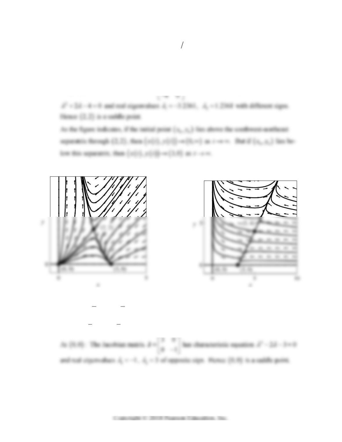
At
3, 0 : The Jacobian matrix 332
02
J has characteristic equation
2560
and negative real eigenvalues 13
, 22
. Hence
3, 0 is a nodal
sink.
At
2, 2 : The Jacobian matrix 21
J has characteristic equation
5
Problem 29
10
Problem 30
30.
11
23
22
11
1
55
x
yx
yx
J
550 Chapter 9: Nonlinear Systems and Phenomena
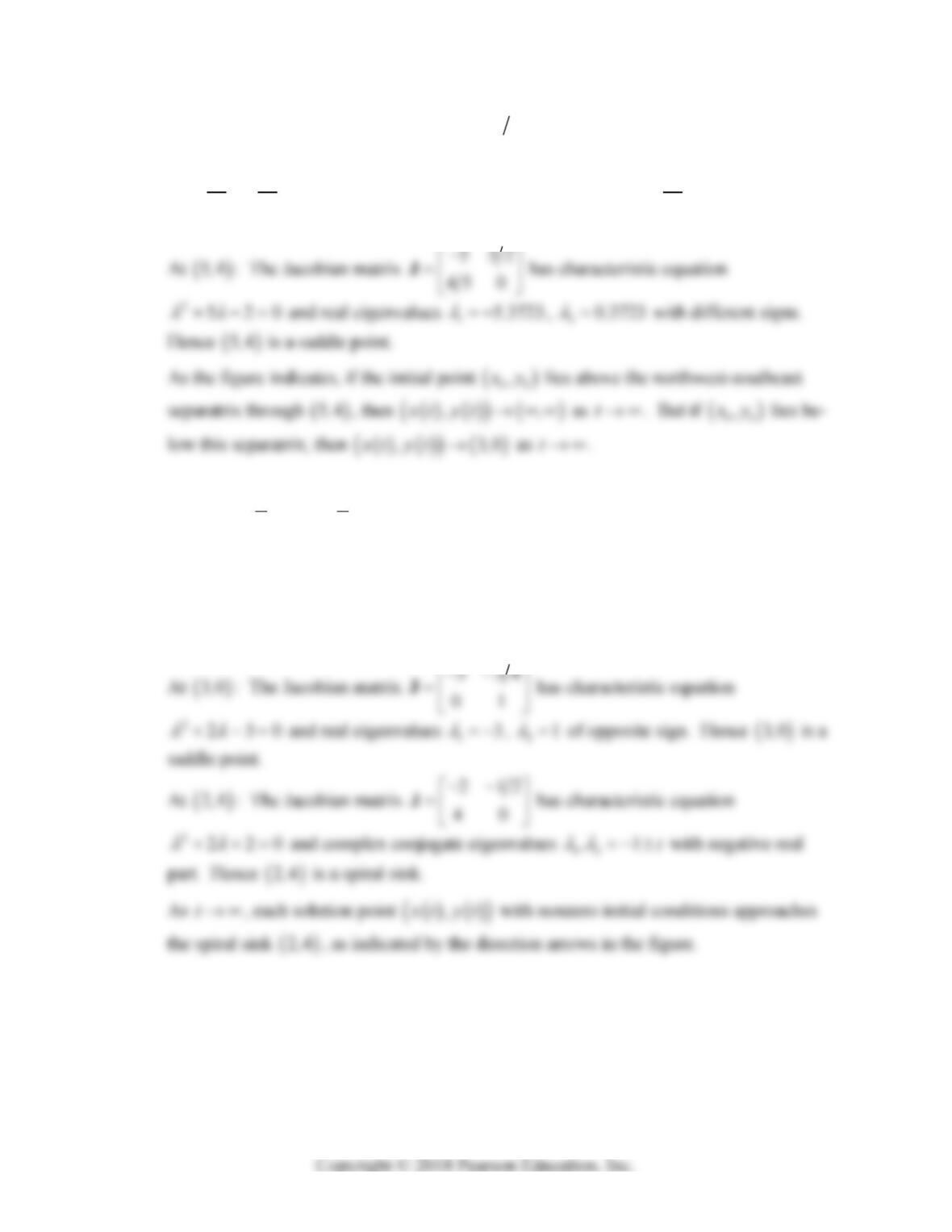
At
3, 0 : The Jacobian matrix 332
02
J has characteristic equation
217 17 0
55
and negative real eigenvalues 13
, 2
17
5
. Hence
3, 0 is a
nodal sink.
31.
11
23
44
2
x
yx
yx
J
At
0, 0 : The Jacobian matrix 30
02
J has characteristic equation 260
and real eigenvalues 12
, 23
of opposite sign. Hence
0, 0 is a saddle point.
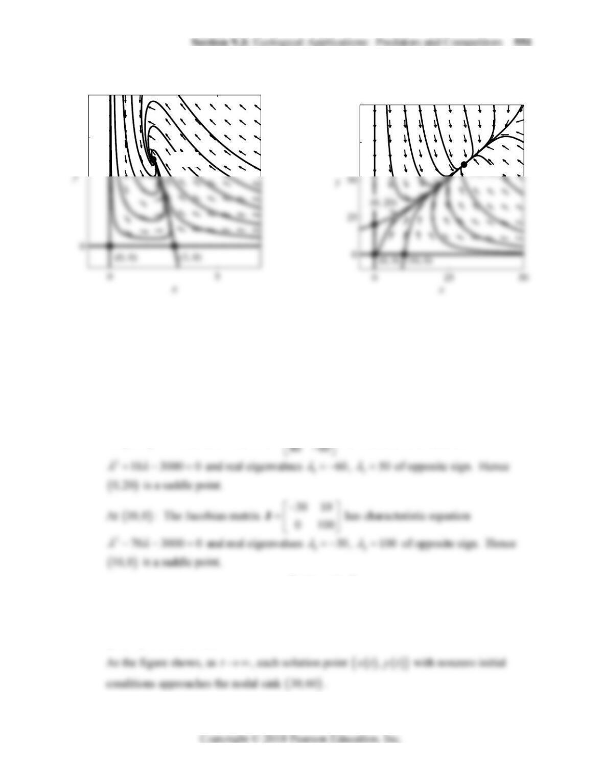
5
(2, 4)
Problem 31
75
100
(30, 60)
Problem 32
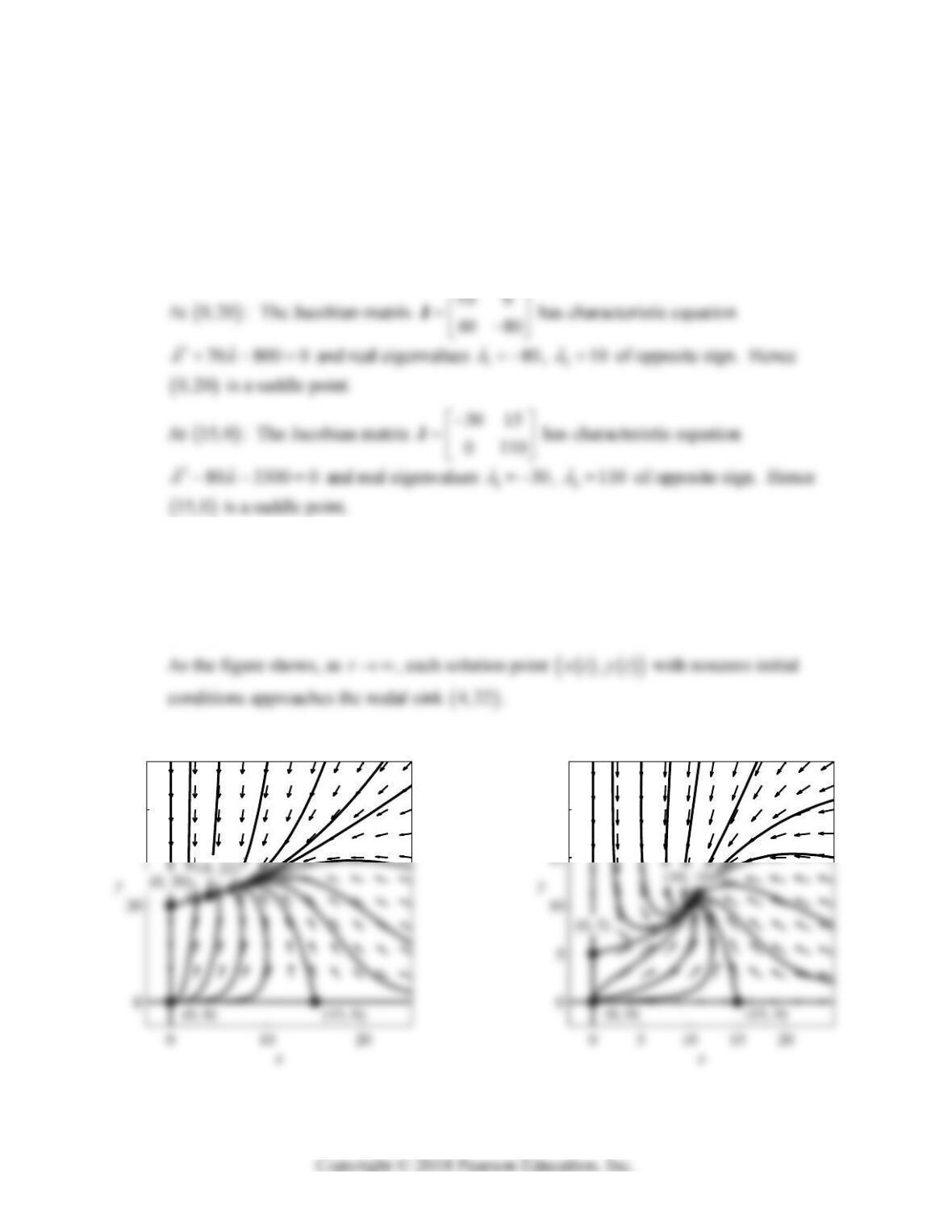
32. 630
44660
xy x
yxy
J
At
0, 0 : The Jacobian matrix 30 0
060
J has characteristic equation
290 1800 0
and positive real eigenvalues 130
, 260
. Hence
0, 0 is a
nodal source.
At
0, 20 : The Jacobian matrix 50 0
J has characteristic equation
At
30,60 : The Jacobian matrix 90 30
240 180
J has characteristic equation
2240 9000 0
and negative real eigenvalues 1231.05
, 238.95
. Hence
30,60 is a nodal sink.
552 Chapter 9: Nonlinear Systems and Phenomena
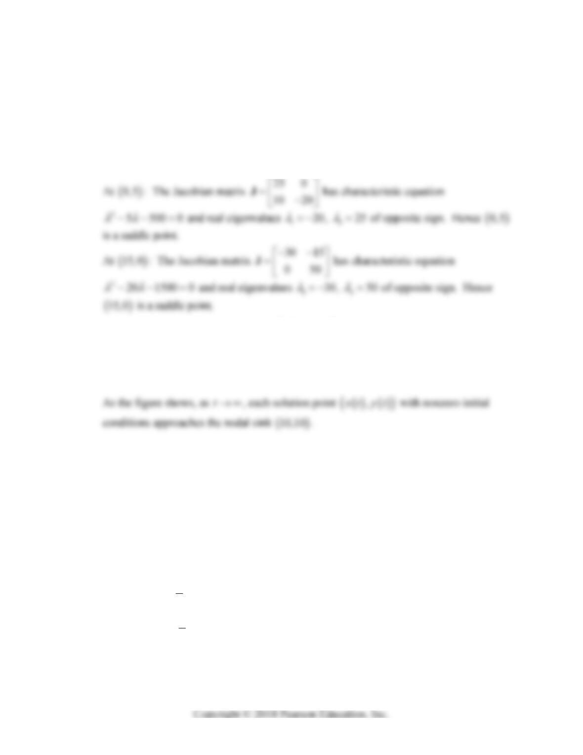
33. 630
44660
xy x
yxy
J
At
0, 0 : The Jacobian matrix 30 0
080
J has characteristic equation
2110 2400 0
and positive real eigenvalues 130
, 280
. Hence
0, 0 is a
nodal source.
At
4, 22 : The Jacobian matrix 84
44 88
J has characteristic equation
296 880 0
and negative real eigenvalues 185.736
, 210.264
. Hence
4, 22 is a nodal sink.
40
Problem 33
20
Problem 34
Section 9.4: Nonlinear Mechanical Systems 553
34. 430
22820
xy x
yxy
J
At
0, 0 : The Jacobian matrix 30 0
020
J has characteristic equation
250 600 0
and positive real eigenvalues 120
, 230
. Hence
0, 0 is a
nodal source.
At
10,10 : The Jacobian matrix 20 10
20 40
J has characteristic equation
260 1000 0
and complex conjugate eigenvalues
12
,3010i
with negative
real part. Hence
10,10 is a spiral sink.
x
SECTION 9.4
NONLINEAR MECHANICAL SYSTEMS
In each of Problems 1–4 we need only substitute the familiar power series for the exponential,
sine, and cosine functions, and then discard all higher-order terms. For each problem we give
the corresponding linear system, the eigenvalues 1
and 2
, and the type of this critical point.
1. 2
1
11 2 2
2
x
xx yxy
3
1
44
6
y
xyy xy
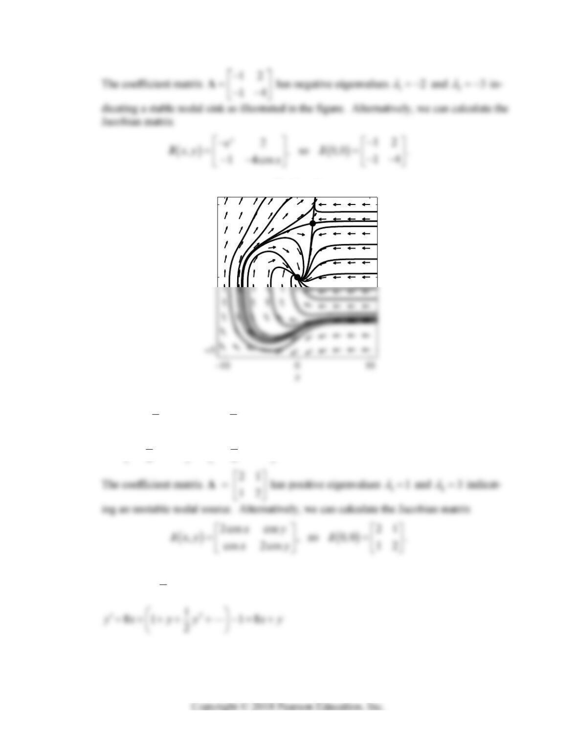
554 Chapter 9: Nonlinear Systems and Phenomena
0
5
y
Problem 1
2. 33
11
22
66
x
xx yy xy
33
11
22
x
x
y
xx yy xy
3. 2
1
1212
2
x
xx y xy
y