41
Quarter Forecast
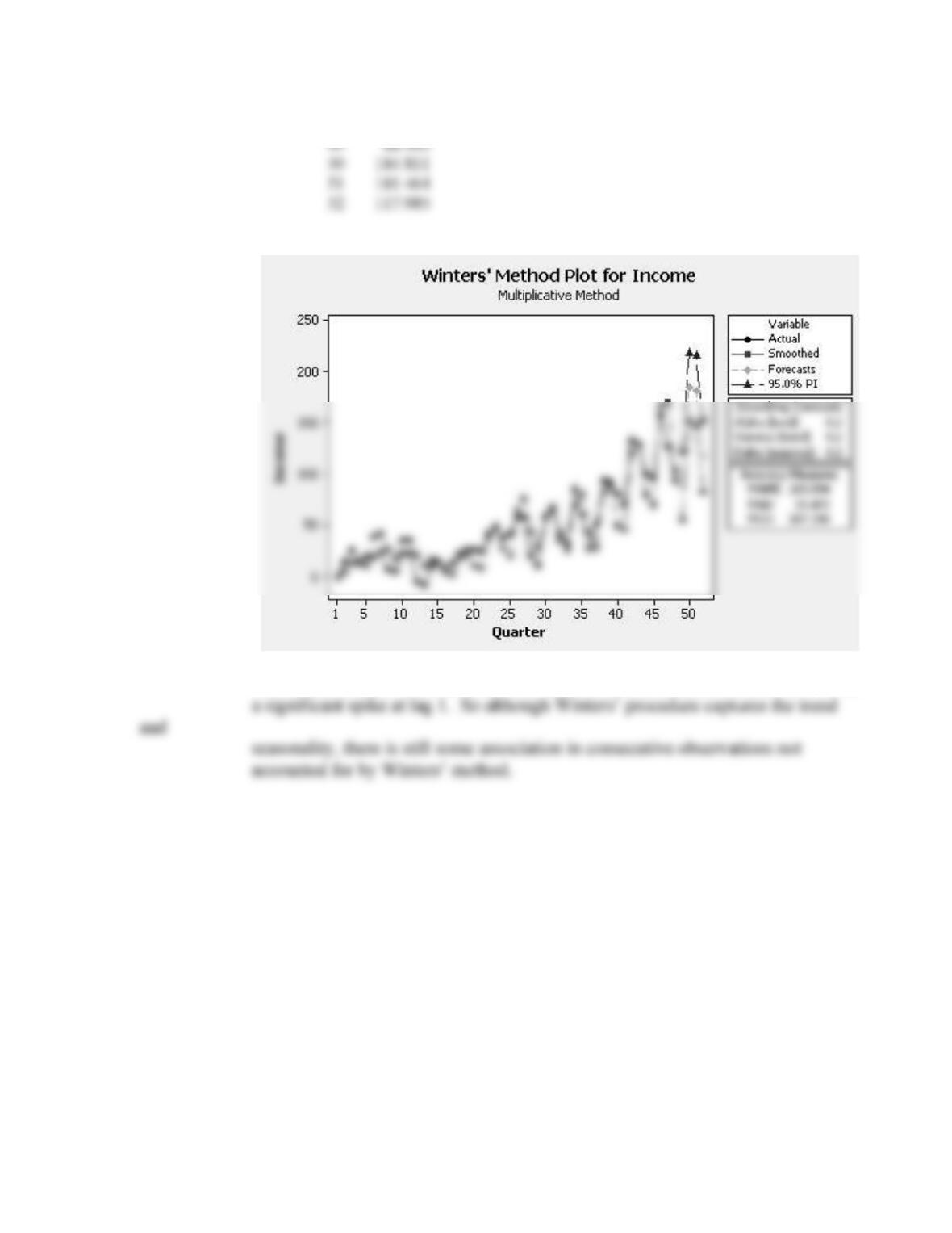
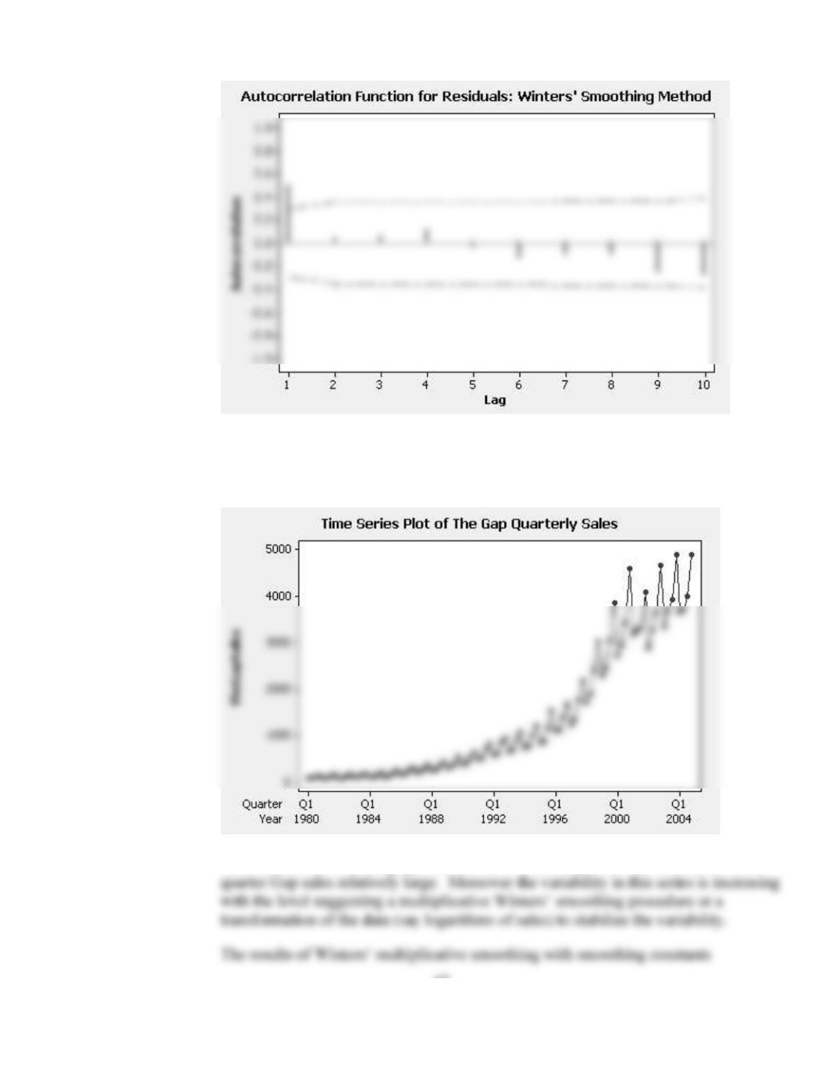
The forecasts seem reasonable but the residual autocorrelation function below has
42
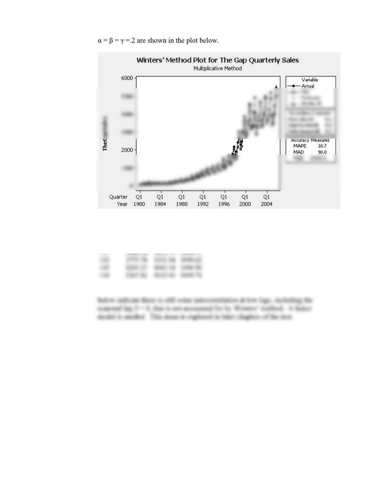
20. A time series plot of The Gap quarterly sales is shown below.
This time series is trending upward and has a seasonal pattern with third and fourth
43
The forecasts for the four quarters of 2005 are:
Forecasts
Quarter Forecast Lower Upper
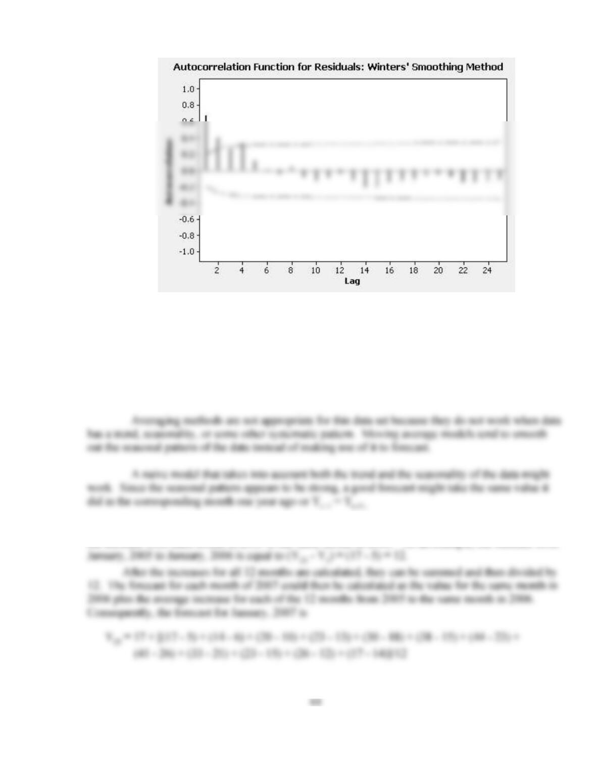
The forecasts seem reasonable, however, the residuals autocorrelations shown
CASE 4-1: THE SOLAR ALTERNATIVE COMPANY
This case provides the student with an opportunity to deal with a frequent real world
problem: small data sets. A plot of the two years of data shows both an upward trend and seasonal
pattern. The forecasting model that is selected must do an accurate job for at least three months into
the future.
However, as it stands, this forecast ignores the trend. One approach to estimate trend is to calculate
the increase from each month in 2005 to the same month in 2006. As an example, the increase from
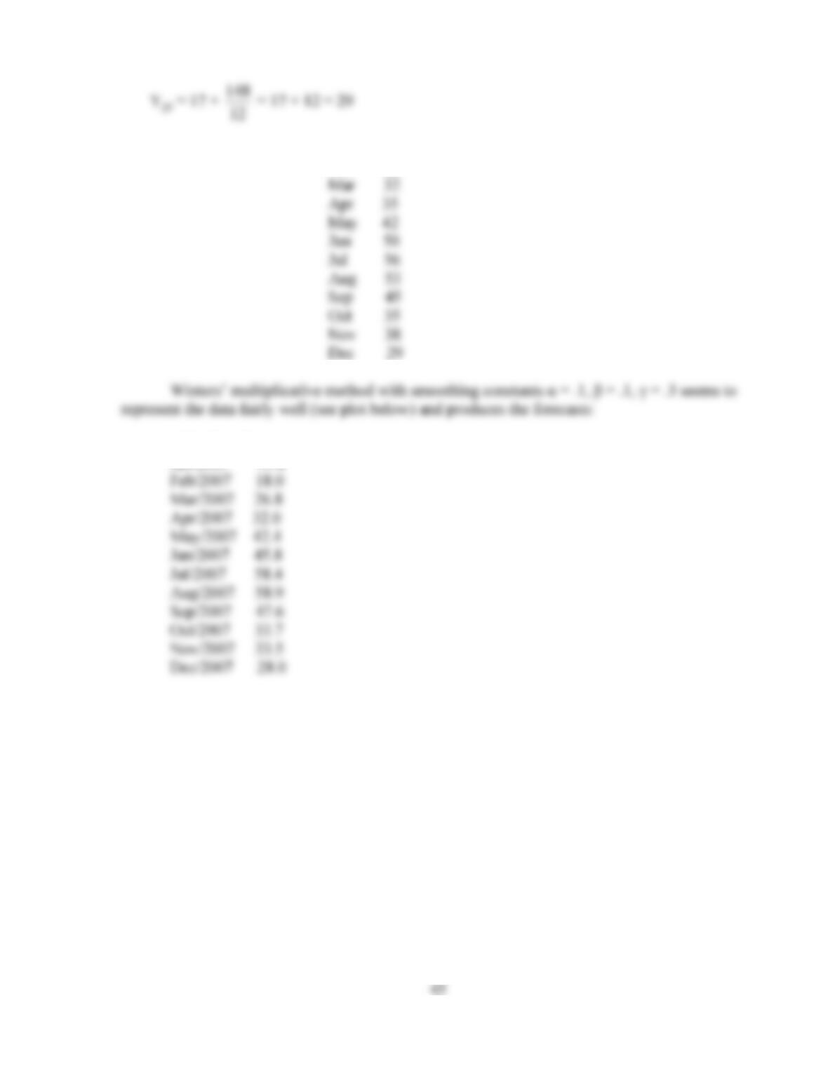
The forecasts for 2007 are: Jan 29
Feb 26
Month Forecast
Jan/2007 19.8
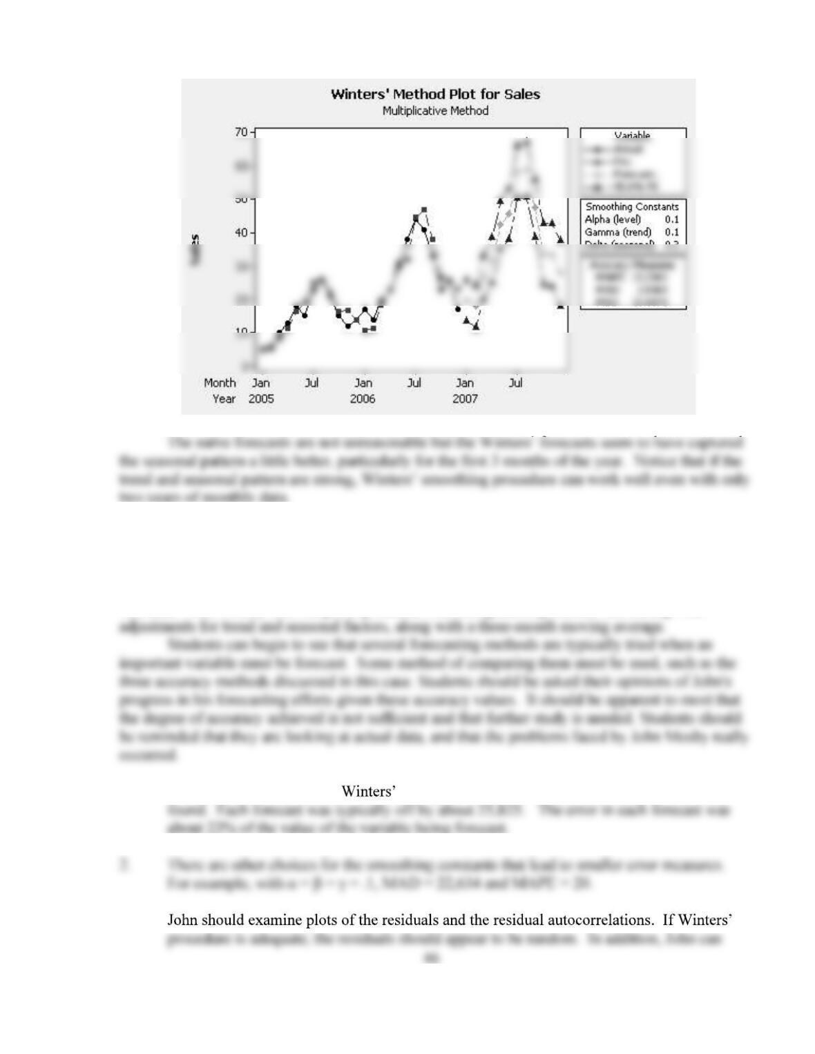
CASE 4-2: MR TUX
This case shows how several exponential smoothing methods can be applied to the Mr.
Tux data. John Mosby tries simple exponential smoothing and exponential smoothing with
1. Of the methods attempted, multiplicative smoothing was the best method John
3.
47
CASE 4-3: CONSUMER CREDIT COUNSELING
1. Students should realize immediately that simply using the basic naive approach of
using last period to predict this period will not allow for forecasts for the rest of
2. A moving average model of any order cannot be defended since any moving average
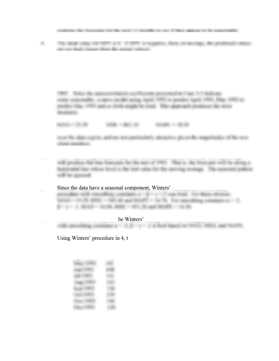
3. multiplicative smoothing
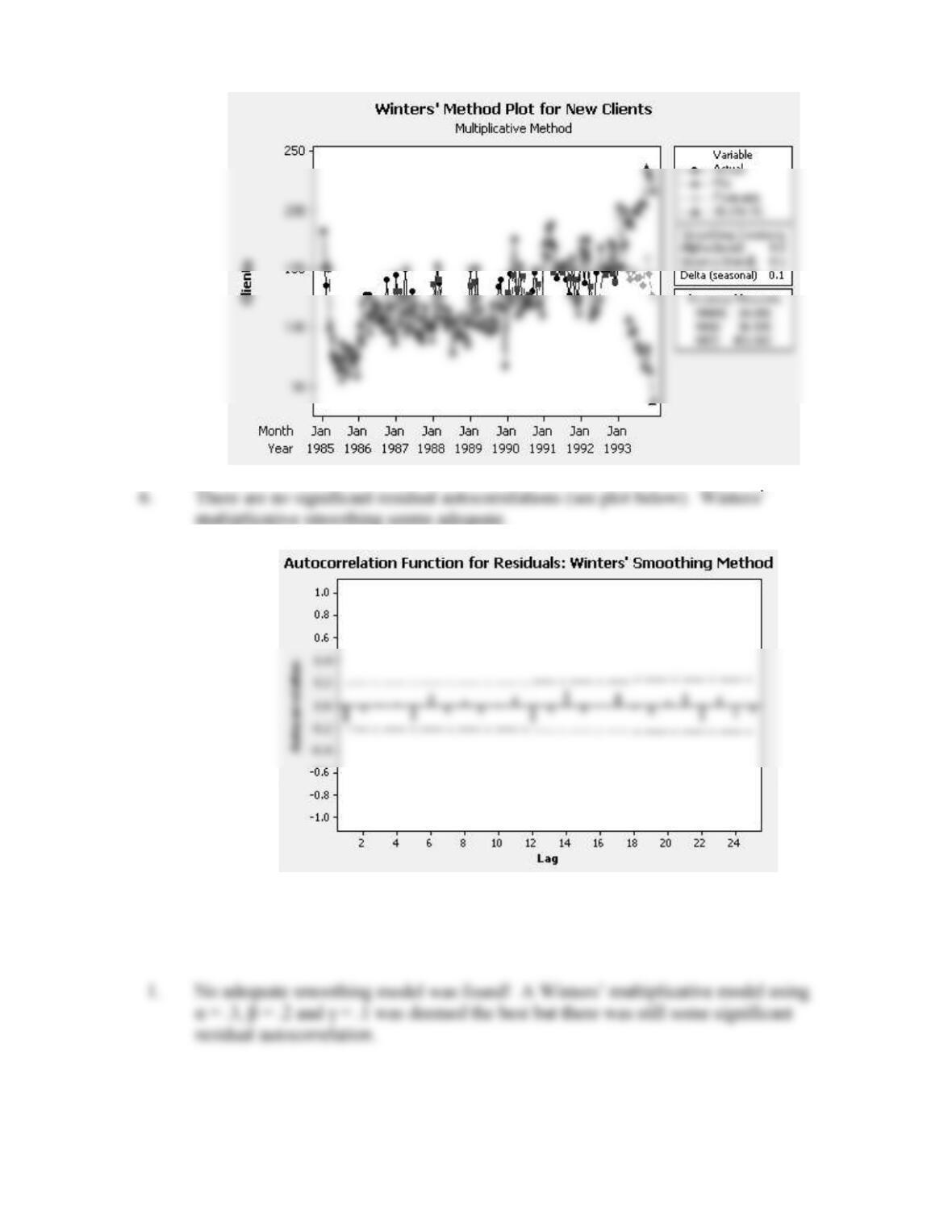
4. Of the methods attempted, t multiplicative smoothing procedure
5. he forecasts for the remainder of 1993 are:
Month Forecast
Apr/1993 148
48
CASE 4-4: MURPHY BROTHERS FURNITURE
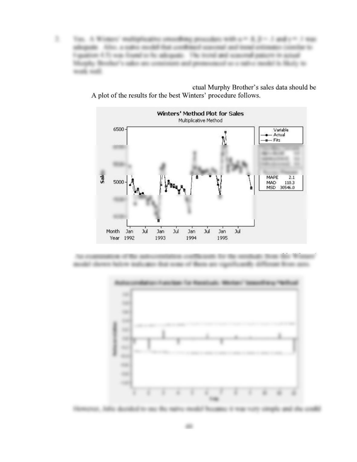
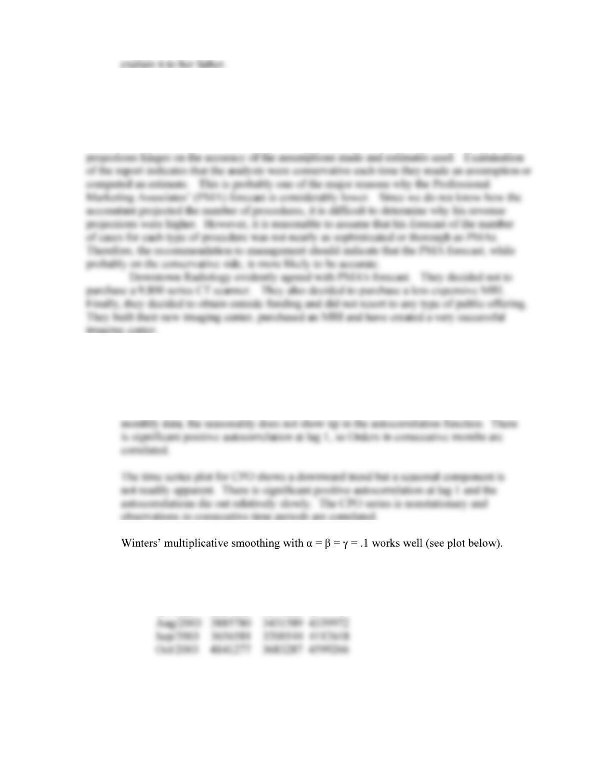
3. Based on the forecasting methods tested, a
used.
50
CASE 4-5: FIVE-YEAR REVENUE PROJECTION FOR DOWNTOWN RADIOLOGY
This case is designed to emphasize the use of subjective probability estimates in a
forecasting situation. The methodology used to generate revenue forecasts is both appropriate
and accurately employed. The key to answering the question concerning the accuracy of the
CASE 4-6: WEB RETAILER
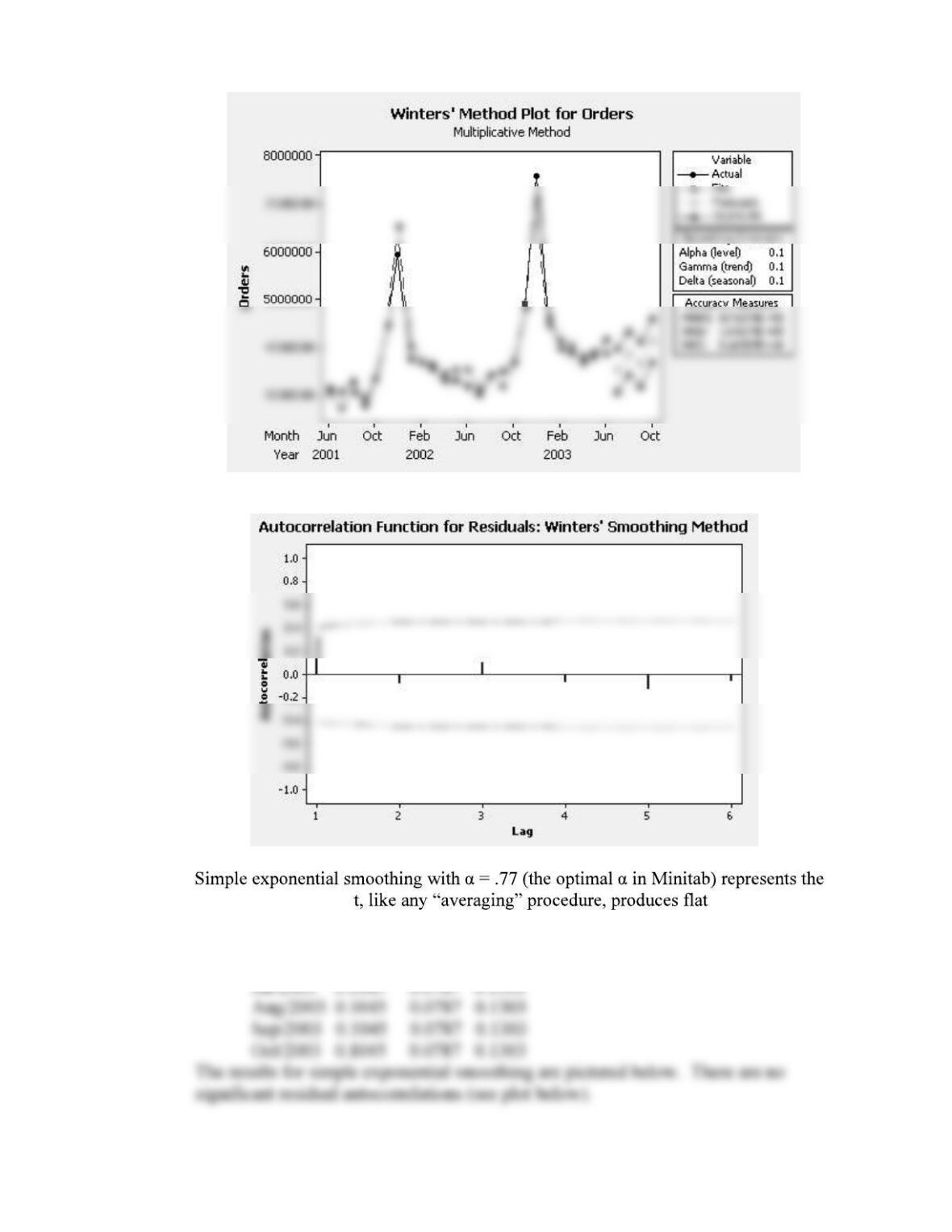
1. The time series plot for Orders shows a slight upward trend and a seasonal pattern
with peaks in December. Because of the relatively small data set, the autocorrelations
are only computed for a limited number of lags, 6 in this case. Consequently with
2.
Forecasts for the next 4 months follow. Residual autocorrelation function below
has no significant autocorrelations.
Month Forecast Lower Upper
Jul/2003 3524720 3072265 3977174
51
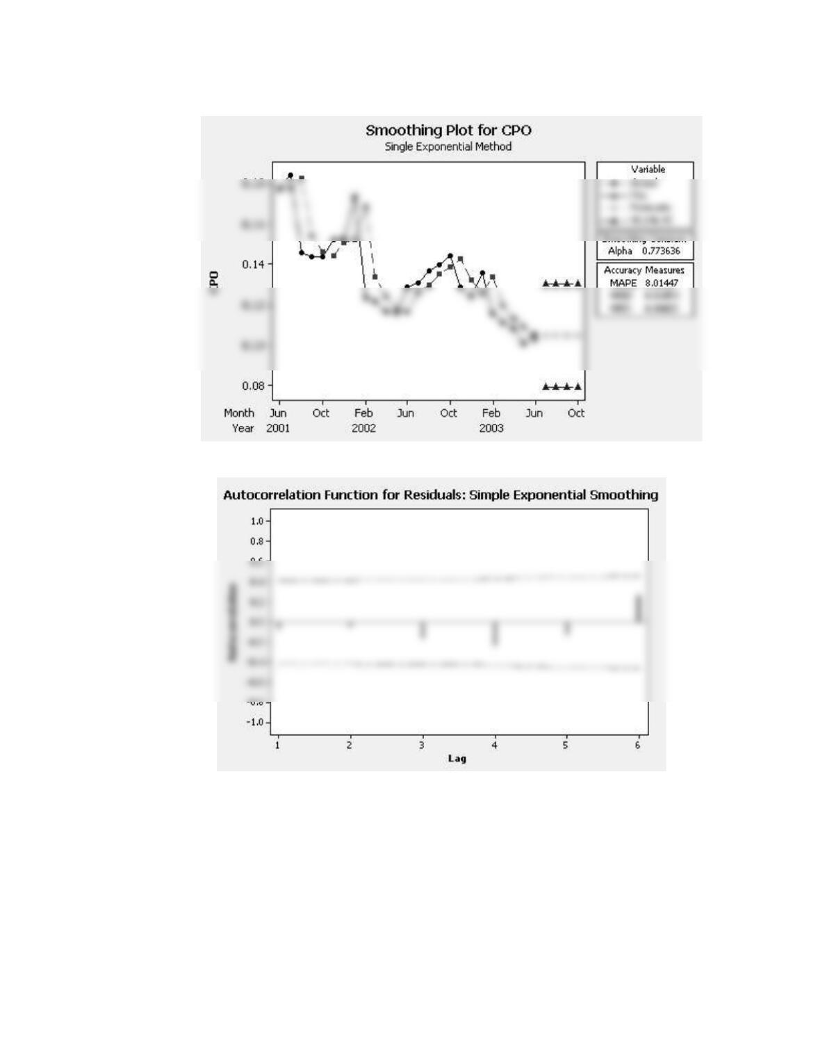
3.
the CPO data well bu -line forecasts.
Forecasts of CPO for the next 4 months are:
Month Forecast Lower Upper
52
4. Multiplying the Orders forecasts in 2 by the CPO forecasts in 3 gives the
Contacts forecasts:
Month Forecast
53
5. It seems reasonable to forecast Contacts directly if the data are available.
6. It may or may not be better to focus on the number of units and contacts per unit
CASE 4-7: SOUTHWEST MEDICAL CENTER
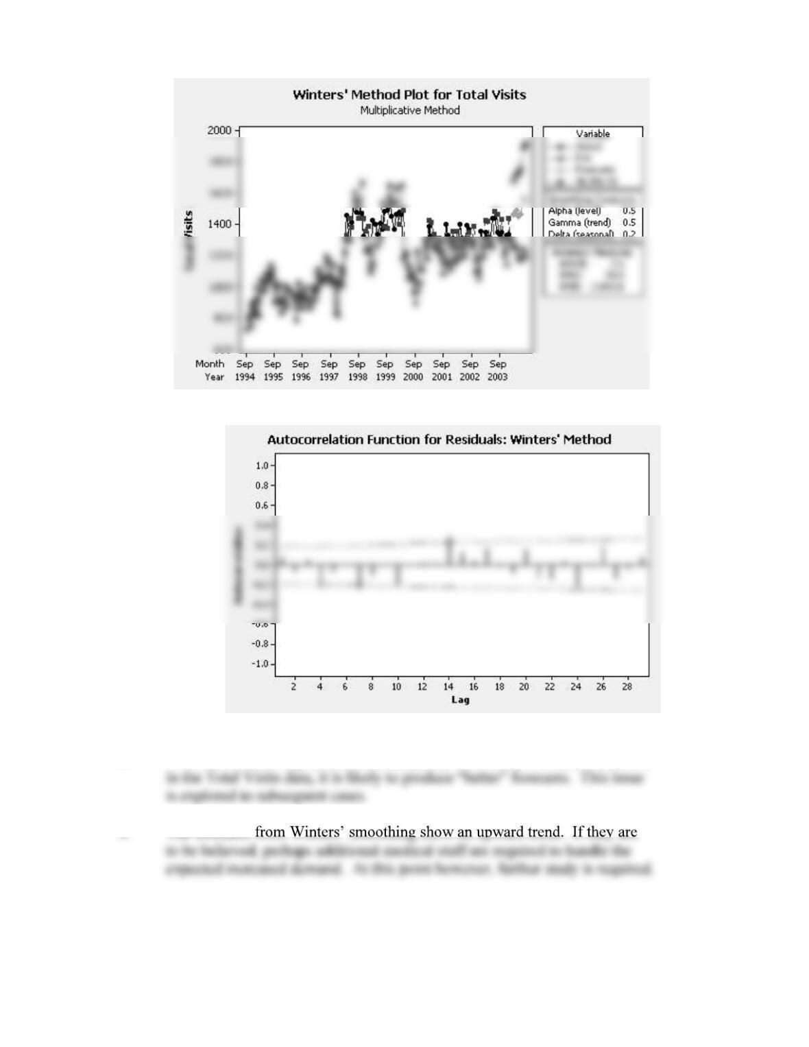
1. Autocorrelation function for total visits suggests time series is nonstationary
2.
Month Forecast Lower Upper
Mar/2004 1465.8 1249.9 1681.7
54
3. If another forecasting method can adequately account for the autocorrelation
55
CASE 4-8: SURTIDO COOKIES
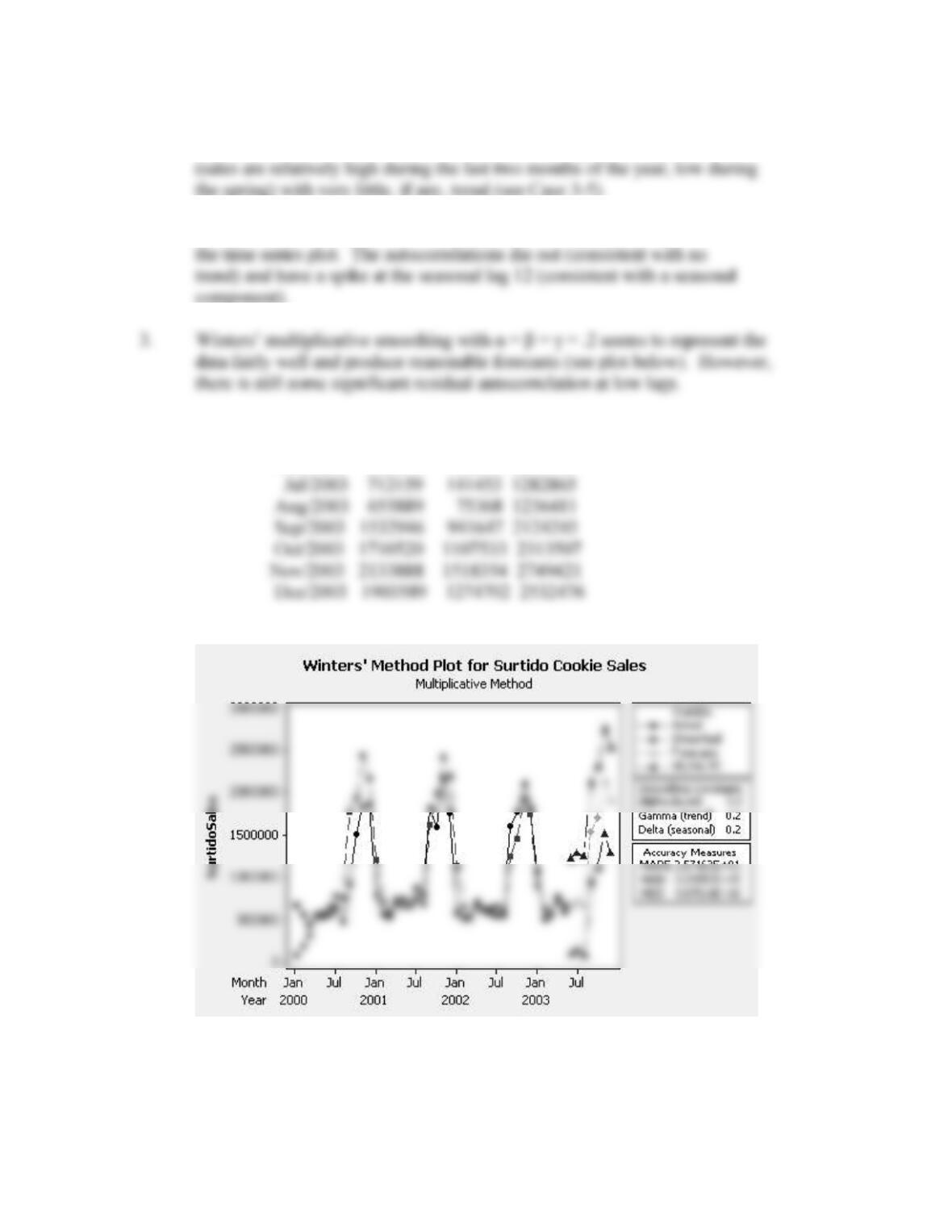
1. Jame learned that Surtido Cookie sales have a strong seasonal pattern
2. The autocorrelation function for sales (see Case 3-5) is consistent with
Month Forecast Lower Upper
Jun/2003 653254 91351 1215157
56
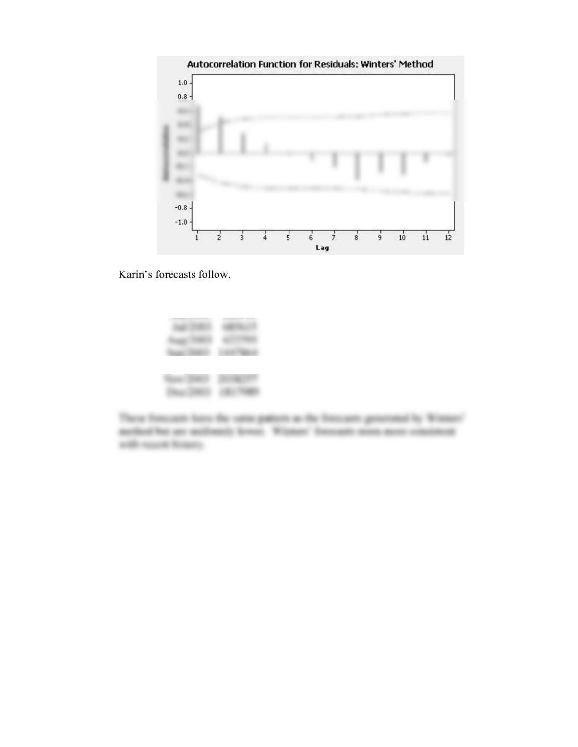
4.
Month Forecast
Jun/2003 618914
Sep/2003 1447864
Oct/2003 1630271