CHAPTER
Discrete Probability Distributions
137
4
4.1 PROBABILITY DISTRIBUTIONS
4.1 Try It Yourself Solutions
1a. (1) measured (2) counted
b. (1) The random variable is continuous because x can be any speed up to the maximum speed of a
space shuttle.
(2) The random variable is discrete because the number of calves born on a farm in one year is
countable.
2ab. c.
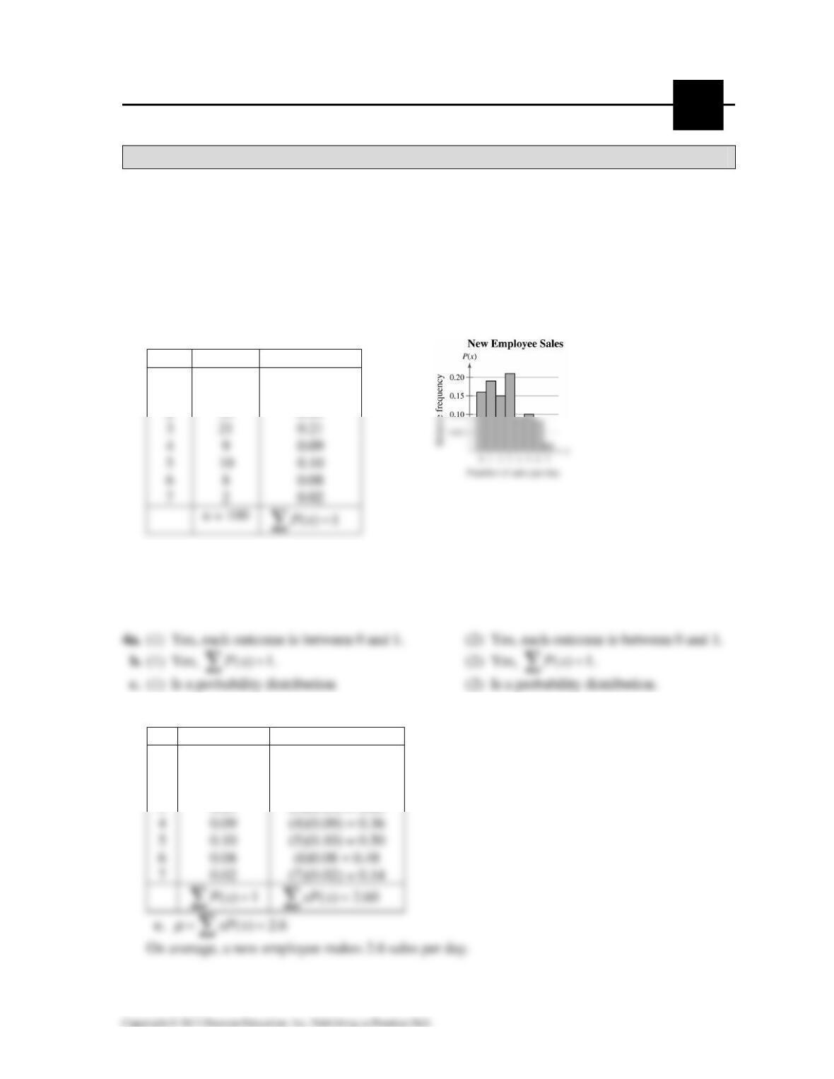
3a. Each P(x) is between 0 and 1.
b. () 1Px =
∑
c. Because both conditions are met, the distribution is a probability distribution.
5ab.
x f P(x)
0 16 0.16
1 19 0.19
2 15 0.15
x P(x) xP(x)
0 0.16 (0)(0.16) = 0.00
1 0.19 (1)(0.19) = 0.19
2 0.15 (2)(0.15) = 0.30
3 0.21 (3)(0.21) = 0.63
138 CHAPTER 4 │ DISCRETE PROBABILITY DISTRIBUTIONS
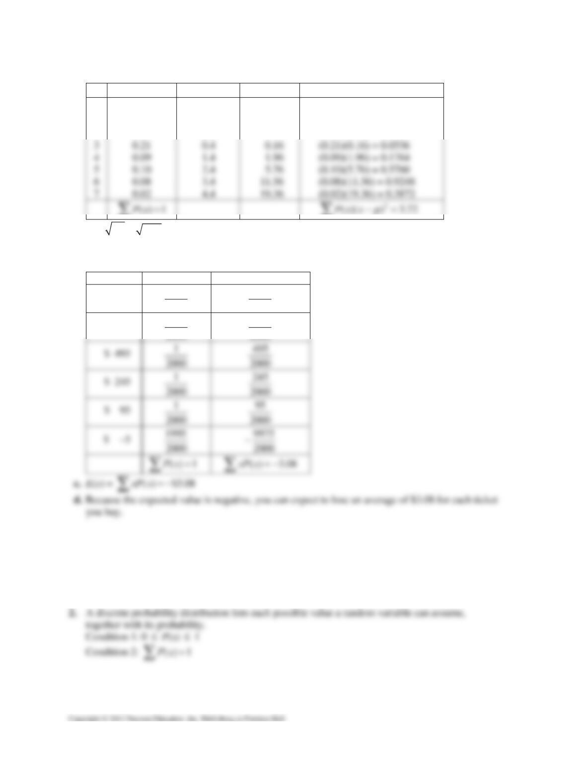
6ab. From 5, 2.6,
µ
−
x f x −
µ
(x −
µ
)2 P(x)(x −
µ
)2
0 0.16 −2.6 6.76 (0.16)(6.76) = 1.0816
1 0.19 −1.6 2.56 (0.19)(2.56) = 0.4864
2 0.15 −0.6 0.36 (0.15)(0.36) = 0.0540
∑ 2
∑
c. 23.72 1.9
σσ
== ≈
d. Most of the data valves differ from the mean by no more than 1.9 sales per day.
7ab.
Gain, x P(x) xP(x)
$1995 1
2000 1995
2000
$ 995 1
2000 995
2000
4.1 EXERCISE SOLUTIONS
1. A random variable represents a numerical value associated with each outcome of a probability
experiment. Examples: Answers will vary.
CHAPTER 4 │ DISCRETE PROBABILITY DISTRIBUTIONS 139
3. No; Expected value may not be a possible value of x for one trial, but it represents the average
value of x over a large number of trials.
7. True
8. False. The expected value of a discrete random variable is equal to the mean of the random
variable.
9. Discrete, because attendance is a random variable that is countable.
10. Continuous, because length of time is a random variable that has an infinite number of possible
outcomes and cannot be counted.
14. Continuous, because the length of time it takes to get to work is a random variable that has an
infinite number of possible outcomes and cannot be counted.
15. Continuous, because the volume of blood drawn for a blood test is a random variable that must be
measured.
16. Discrete, because the number of tornadoes in the month of June in Oklahoma is a random
variable that is countable.
140 CHAPTER 4 │ DISCRETE PROBABILITY DISTRIBUTIONS
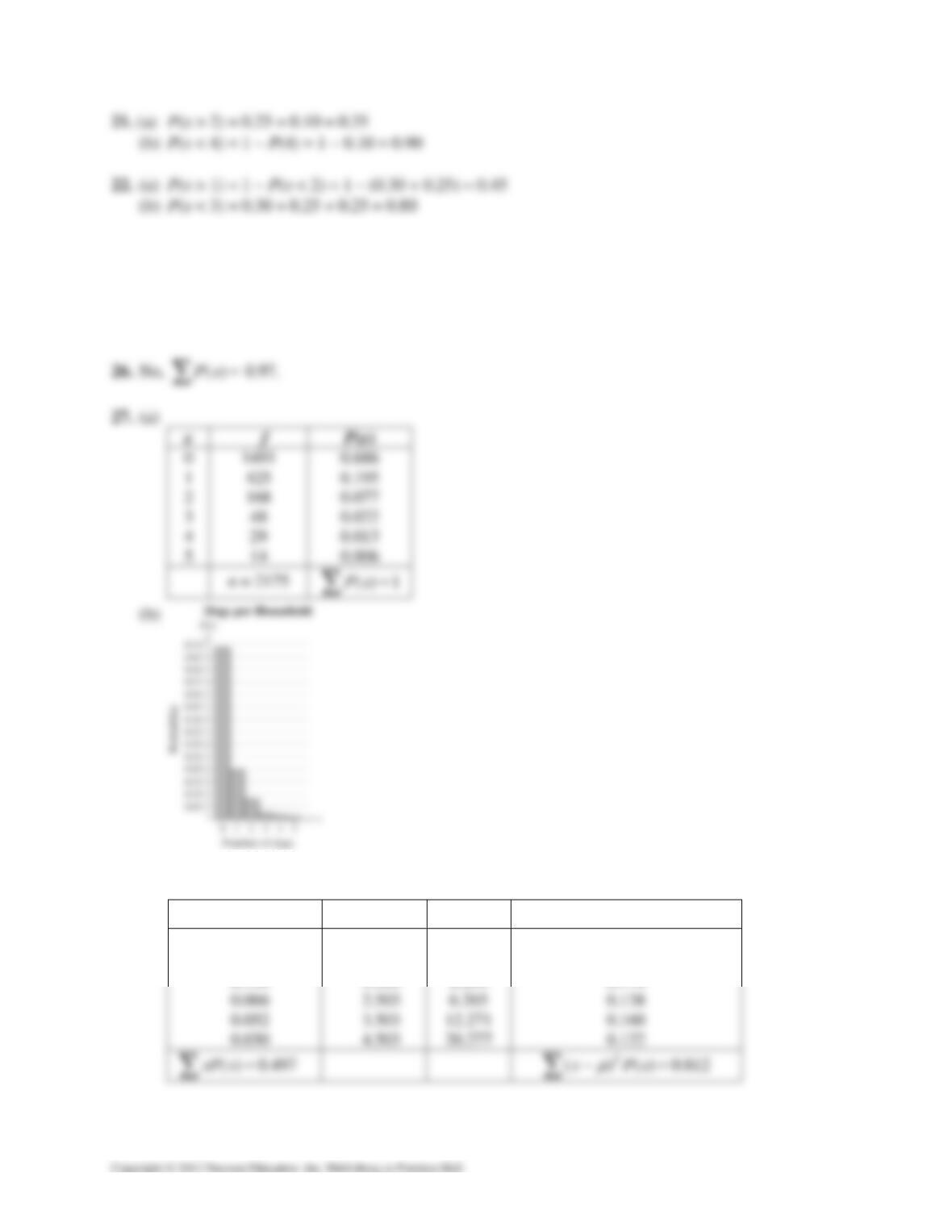
23. ( ) 1 (3) 0.22Px P=→ =
∑ 24. ( ) 1 (1) 0.15Px P=→ =
∑
25. Because each P(x) is between 0 and 1, and () 1,Px =
∑ the distribution is a probability
distribution.
Skewed right
(c)
xP(x) (x −
µ
) (x −
µ
)2 (x −
µ
)2P(x)
0 −0.497 0.247 0.169
0.195 0.503 0.253 0.049
0.154 1.503 2.259 0.174
CHAPTER 4 │ DISCRETE PROBABILITY DISTRIBUTIONS 141
28. (a)
x f P(x)
4 20 0.190
5 23 0.219
6 23 0.219
7 36 0.343
8 3 0.029
n = 105 () 1Px =
∑
(c)
xP(x) (x −
µ
) (x −
µ
)2 (x −
µ
)2P(x)
0.760 −1.802 3.247 0.617
1.095 −0.802 0.643 0.141
1.314 0.198 0.039 0.009
2.401 1.198 1.435 0.492
0.232 2.198 4.831 0.140
( ) 5.802xP x =
∑
2
( ) ( ) 1.399xPx
µ
−=
∑
142 CHAPTER 4 │ DISCRETE PROBABILITY DISTRIBUTIONS
29. (a)
x f P(x)
0 26 0.01
(b)
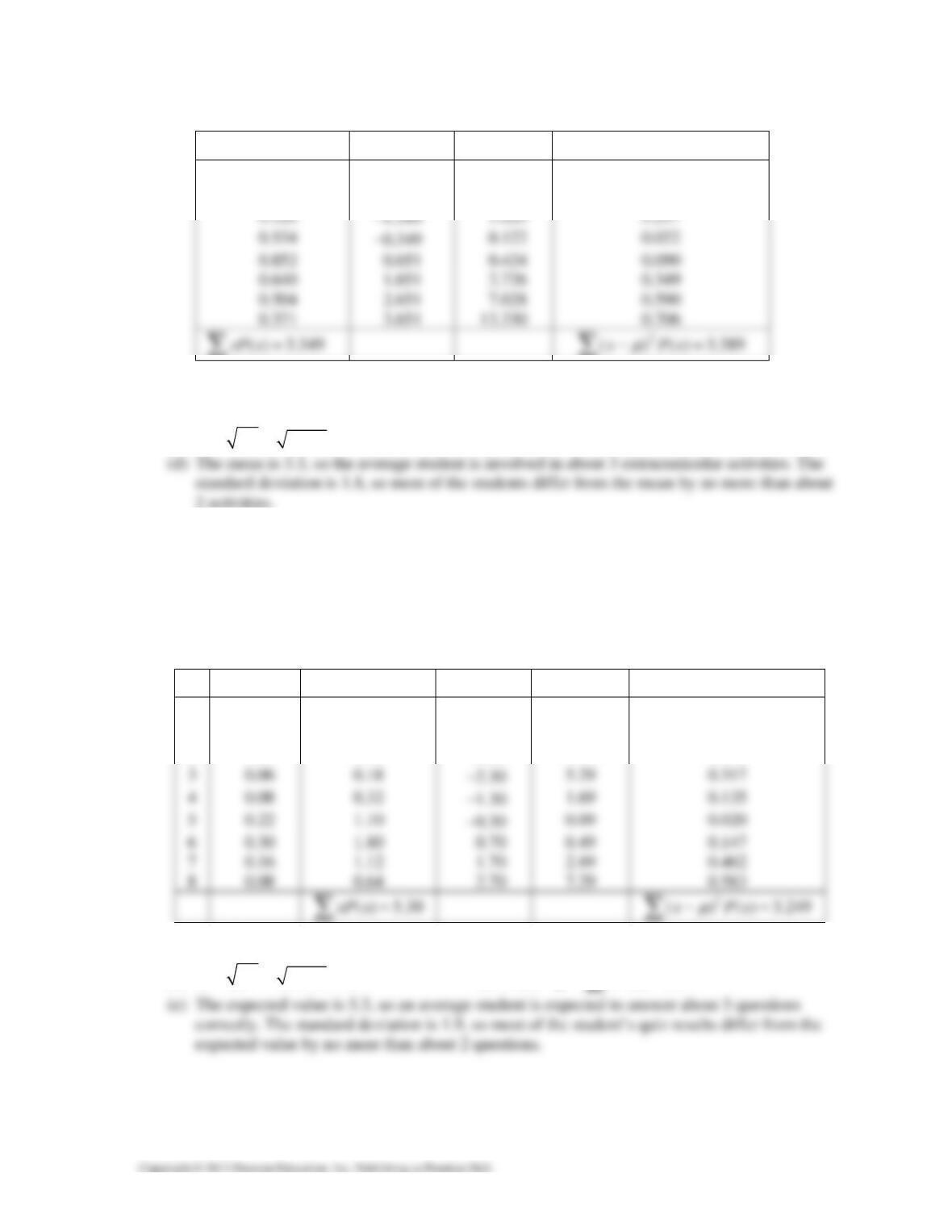
Skewed left
(c)
xP(x) (x −
µ
) (x −
µ
)2 (x −
µ
)2P(x)
0.00 −2.35 5.523 0.055
30. (a)
x f P(x)
0 95 0.250
1 113 0.297
CHAPTER 4 │ DISCRETE PROBABILITY DISTRIBUTIONS 143
(b)
Skewed right
(c)
xP(x) (x −
µ
) (x −
µ
)2 (x −
µ
)2P(x)
0 −1.5 2.25 0.563
0.297 −0.5 0.25 0.074
0.458 0.5 0.25 0.057
0.504 1.5 2.25 0.378
31. (a)
x f P(x)
0 6 0.031
1 12 0.063
2 29 0.151
144 CHAPTER 4 │ DISCRETE PROBABILITY DISTRIBUTIONS
(c)
xP(x) (x −
µ
) (x −
µ
)2 (x −
µ
)2P(x)
0 −3.41 11.628 0.360
0.063 −2.41 5.808 0.366
0.302 −1.41 1.988 0.300
( ) 3.410 3.4xP x
µ
==≈
∑
22
( ) ( ) 2.103 2.1xPx
σµ
=− =≈
∑
22.103 1.5
σσ
== ≈
32. (a)
x f P(x)
0 19 0.059
1 39 0.122
2 52 0.163
(b)
CHAPTER 4 │ DISCRETE PROBABILITY DISTRIBUTIONS 145
(c)
xP(x) (x −
µ
) (x −
µ
)2 (x −
µ
)2P(x)
0 −3.349 11.216 0.662
0.122 −2.349 5.518 0.673
( ) 3.349 3.3xP x
µ
==≈
∑
22
( ) ( ) 3.389 3.4xPx
σµ
=− =≈
∑
23.389 1.8
σσ
== ≈
33. An expected value of 0 means that the money gained is equal to the spent, representing the
breakeven point.
34. A “fair bet” in a game of chance has an expected value of 0, which means that the chances of
losing are equal to the chances of winning.
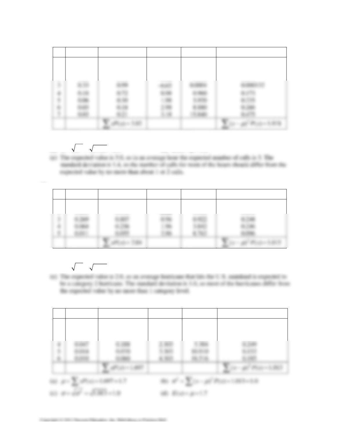
35.
x P(x) xP(x) (x −
µ
) (x −
µ
)2 (x −
µ
)2P(x)
0 0.02 0.00 −5.30 28.09 0.562
1 0.02 0.02 −4.30 18.49 0.370
2 0.06 0.12 −3.30 10.89 0.653
(a) () 5.3xP x
µ
==
∑ (b)
22
( ) ( ) 3.249 3.3xPx
σµ
=− =≈
∑
(c) 23.249 1.9
σσ
== ≈ (d) () () 5.3Ex xPx
µ
== =
∑
146 CHAPTER 4 │ DISCRETE PROBABILITY DISTRIBUTIONS
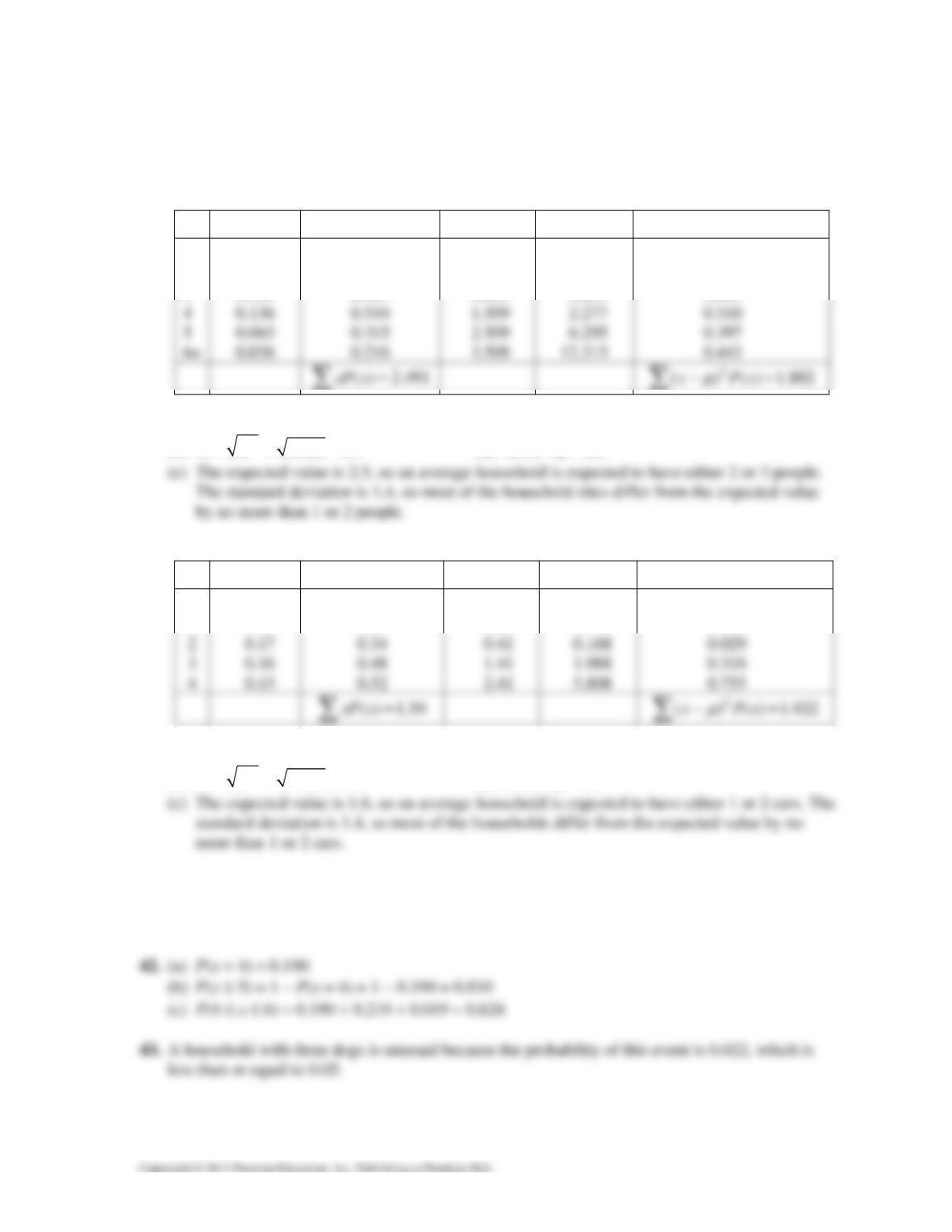
36.
x P(x) xP(x) (x −
µ
) (x −
µ
)2 (x −
µ
)2P(x)
0 0.01 0 −3.02 9.120 0.091
1 0.10 0.10 −2.02 4.080 0.408
2 0.26 0.52 −1.02 1.040 0.270
(a) ( ) 3.02 3.0xP x
µ
==≈
∑ (b)
22
()()1.9181.9xPx
σµ
=− =≈
∑
(c) 21.918 1.4
σσ
== ≈ (d) () 3.0Ex
µ
==
37.
x P(x) xP(x) (x −
µ
) (x −
µ
)2 (x −
µ
)2P(x)
1 0.392 0.392 −1.04 1.082 0.424
2 0.265 0.530 −0.04 0.002 0.001
(a) ( ) 2.04 2.0xP x
µ
==≈
∑ (b)
22
()()1.0151.0xPx
σµ
=− =≈
∑
(c) 21.015 1.0
σσ
== ≈ (d) () 2.0Ex
µ
==
38.
x P(x) xP(x) (x −
µ
) (x −
µ
)2 (x −
µ
)2P(x)
1 0.555 0.555 −0.697 0.486 0.270
2 0.298 0.596 0.303 0.092 0.027
3 0.076 0.228 1.303 1.698 0.129
CHAPTER 4 │ DISCRETE PROBABILITY DISTRIBUTIONS 147
(e) The expected value is 1.7, so an average car crossing the Tacoma Narrows Bridge is expected
to have either 1 or 2 people in it. The standard deviation is 1.0, so most of the car occupancies
differ from the expected value by no more than 1 occupant.
39.
x P(x) xP(x) (x −
µ
) (x −
µ
)2 (x −
µ
)2P(x)
1 0.275 0.275 −1.491 2.223 0.611
2 0.332 0.664 −0.491 0.241 0.080
3 0.159 0.447 0.509 0.259 0.041
(a) ( ) 2.491 2.5xP x
µ
==≈
∑ (b)
22
( ) ( ) 1.882 1.9xPx
σµ
=− =≈
∑
(c) 21.882 1.4
σσ
== ≈ (d) () 2.5Ex
µ
==
40.
x P(x) xP(x) (x −
µ
) (x −
µ
)2 (x −
µ
)2P(x)
0 0.29 0 −1.59 2.528 0.733
1 0.25 0.25 −0.59 0.348 0.087
(a) ( ) 1.59 1.6xP x
µ
==≈
∑ (b)
22
( ) ( ) 1.922 1.9xPx
σµ
=− =≈
∑
(c) 21.922 1.4
σσ
== ≈ (d) () 1.6Ex
µ
==
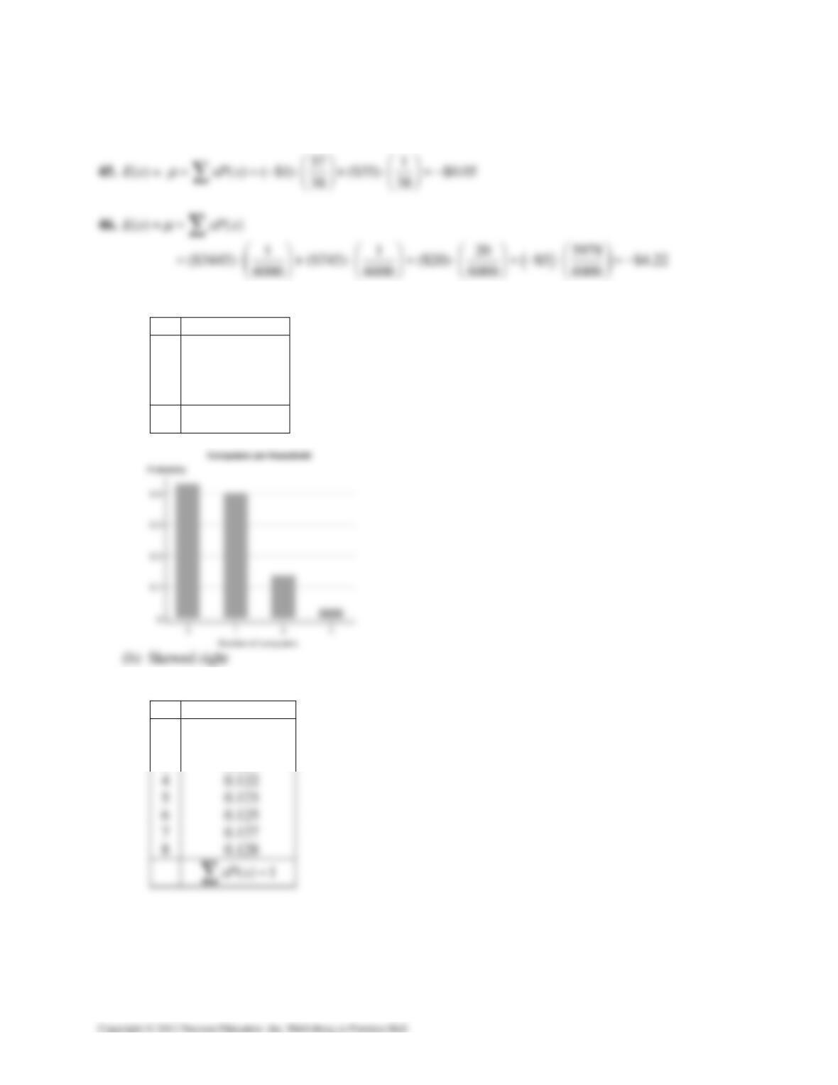
41. (a) P(x < 2) = 0.686 + 0.195 = 0.881
(b) P(x ≥ 1) = 1 − P(x = 0) = 1 − 0.686 = 0.314
(c) P(1 ≤ x ≤ 3) = 0.195 + 0.077 + 0.022 = 0.294
148 CHAPTER 4 │ DISCRETE PROBABILITY DISTRIBUTIONS
44. A World Series in which eight games were played is unusual because the probability of this event
is 0.029, which is less than 0.05.
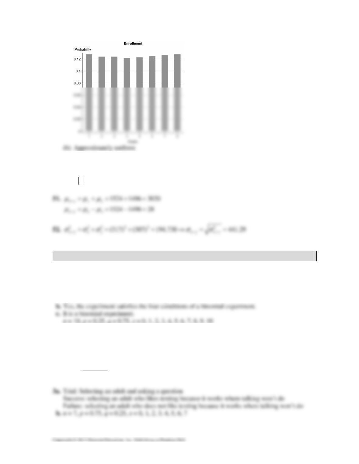
47. (a)
48. (a)
x P(x)
1 0.128
2 0.124
3 0.124
x P(x)
0 0.432
1 0.403
2 0.137
3 0.029
() 1xP x =
∑
CHAPTER 4 │ DISCRETE PROBABILITY DISTRIBUTIONS 149
49. 1000 1.05(36,000) $38,800
xx
ab=+ = + =
µ
µ
50. (1.04)(3899) $4054.96
yx
b
σσ
== =
4.2 BINOMIAL DISTRIBUTIONS
4.2 Try It Yourself Solutions
1a. Trial answering a question
Success: the question answered correctly
2a. Trial: drawing a card with replacement
Success: card drawn is a club
Failure: card drawn is not a club
b. n = 5, p = 0.25, q = 0.75, x = 3
c. P(3) = 32
5! (0.25) (0.75) 0.088
(5 3)!3! ≈
−
150 CHAPTER 4 │ DISCRETE PROBABILITY DISTRIBUTIONS
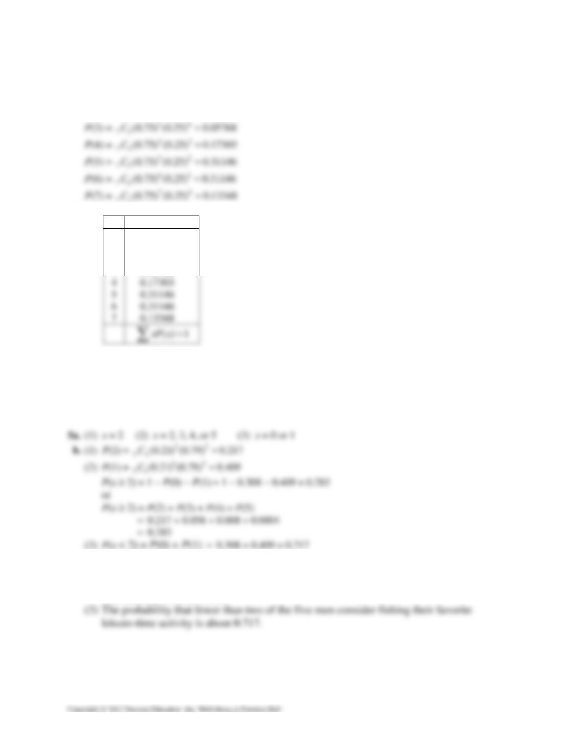
c. P(0) = 07
70
(0.75) (0.25) 0.00006C≈
P(1) = 16
71
(0.75) (0.25) 0.00128C≈
P(2) = 25
72
(0.75) (0.25) 0.01154C≈
d.
x P(x)
0 0.00006
1 0.00128
2 0.01154
3 0.05768
4a. n = 250, p = 0.71, x = 178
b. P(178) ≈ 0.056
c. The probability that exactly 178 people from a random sample of 250 people in the United States
will use more than one topping on their hot dog is about 0.056.
d. Because 0.056 is not less than or equal to 0.05, this event is not unusual.
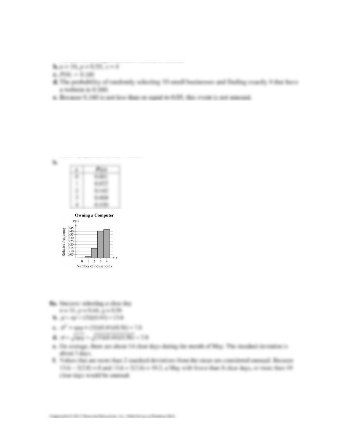
c. (1) The probability that exactly two of the five men consider fishing their favorite
leisure-time activity is about 0.217.
(2) The probability that at least two of the five men consider fishing their favorite leisure-
time activity is about 0.283.
CHAPTER 4 │ DISCRETE PROBABILITY DISTRIBUTIONS 151
6a. Trial: Selecting a business and asking if it has a website
Success: Selecting a business with a website
Failure: Selecting a business without a website
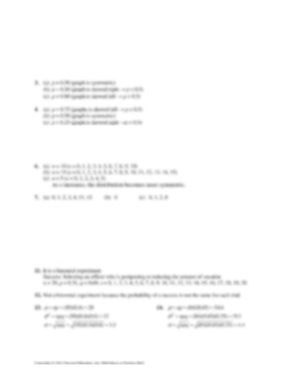
7a. P(0) = 04
40
(0.81) (0.19) 0.001C≈
P(1) = 13
41
(0.81) (0.19) 0.022C≈
P(2) = 22
42
(0.81) (0.19) 0.142C≈
P(3) = 31
43
(0.81) (0.91) 0.404C≈
P(4) = 40
(0.81) (0.19) 0.430C≈
c.
Skewed left
d. Yes, it would be unusual if exactly zero or exactly one of the four households owned a computer,
because each of these events has a probability that is less than 0.05.
152 CHAPTER 4 │ DISCRETE PROBABILITY DISTRIBUTIONS
4.2 EXERCISE SOLUTIONS
1. Each trial is independent of the other trials if the outcome of one trial does not affect the outcome
of any of the other trials.
2. The random variable measures the number of successes in n trials.
5. (a) n = 12 (x = 0, 1, 2, 3, 4, 5, 6, 7, 8, 9, 10, 11, 12)
(b) n = 4 (x = 0, 1, 2, 3, 4)
(c) n = 8 (x = 0, 1, 2, 3, 4, 5, 6, 7, 8)
As n increases, the distribution becomes more symmetric.
8. (a) 0, 1, 2, 3, 4 (b) 0, 1, 2, 3, 4, 5, 6, 7, 8, 15 (c) 0, 1
9. It is a binomial experiment.
Success: baby recovers
n = 5, p = 0.80, q = 0.20, x = 0, 1, 2, 3, 4, 5
10. It is a binomial experiment.
Success: person does not make a purchase
n = 18, p = 0.74, q = 0.26, x = 0, 1, 2, 3, 4, 5, 6, 7, 8, 9, 10, 11, 12, 13, 14, 15, 16, 17, 18
CHAPTER 4 │ DISCRETE PROBABILITY DISTRIBUTIONS 153
15. (124)(0.26) 32.2np
µ
== = 16. (316)(0.82) 259.1np
µ
== =
2(124)(0.26)(0.74) 23.9npq
σ
== = 2(316)(0.82)(0.18) 46.6npq
σ
== =
(124)(0.26)(0.74) 4.9npq
σ
== ≈ (316)(0.82)(0.18) 6.8npq== ≈
σ
18. n = 7, p = 0.7
(a) P(5) ≈ 0.318
(b) P(x ≥ 5) = P(5) + P(6) + P(7) ≈ 0.318 + 0.247 + 0.082 = 0.647
(c) P(x < 5) = 1 − P(x ≥ 5) ≈ 1 − 0.647 = 0.353
19. n = 10, p = 0.59
20. n = 12, p = 0.1
(a) P(4) ≈ 0.021
(b) P(x ≥ 4) = 1 − P(x < 4) = 1 − P(0) − P(1) − P(2) − P(3)
≈ 1 − 0.282 − 0.377 − 0.230 − 0.085 = 0.026
(c) P(x < 4) = 1 − P(x ≥ 4) ≈ 1 − 0.026 = 0.974
21. n = 8, p = 0.55
22. n = 20, p = 0.7
(a) P(1) ≈ 1.627 × 9
10−
(b) P(x > 1) = 1 − P(x ≤ 1) = 1 − P(0) − P(1)
11 9
1 3.487 10 1.627 10 0.9999999983
−−
≈− × − × ≈
(c) P(x ≤ 1) = P(0) + P(1) ≈ 11 9 9
3.487 10 1.627 10 1.662 10
−−−
×+ ×≈ ×
154 CHAPTER 4 │ DISCRETE PROBABILITY DISTRIBUTIONS
25. n = 10, p = 0.28
(a) P(2) ≈ 0.255
(b) P(x > 2) = 1 − P(x ≤ 2) = 1 − (P(0) + P(1) + P(2))
≈ 1 − (0.037 + 0.146 + 0.255)
≈ 0.562
(c) P(x ≤ 2 ≤ 5) = P(2) + P(3) + P(4) + P(5)
≈ 0.255 + 0.264 + 0.180 + 0.084
= 0.783
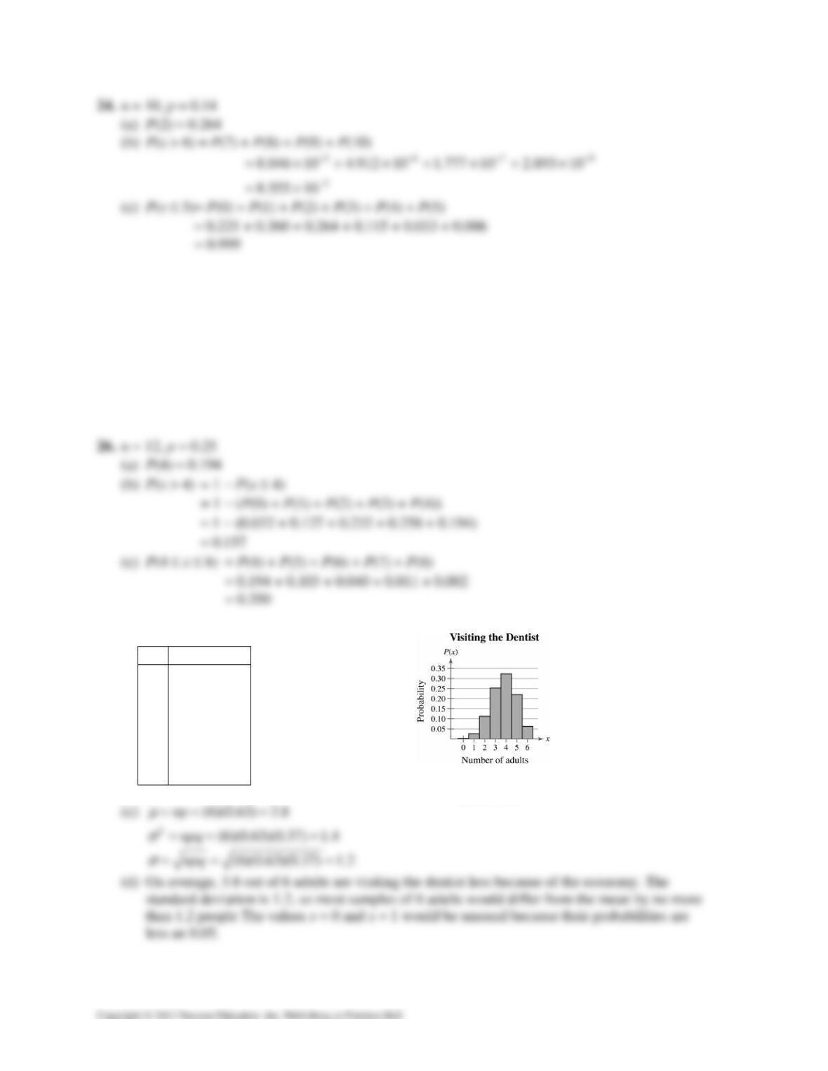
27. (a) n = 6, p = 0.63 (b)
Skewed left
x P(x)
0 0.003
1 0.026
2 0.112
3 0.253
4 0.323
5 0.220
6 0.063