
23
The problems in this chapter focus mainly on the utility maximization assumption. Relatively
simple computational problems (mainly based on Cobb–Douglas and CES utility functions)
are included. Comparative statics exercises are included in a few problems, but for the most
part, introduction of this material is delayed until Chapters 5 and 6.
Comments on Problems
4.1 This problem is a simple Cobb–Douglas example. Part (b) asks students to compute
income compensation for a price rise and may prove difficult for them. As a hint,
they might be told to find the correct bundle on the original indifference curve first,
and then compute its cost.
4.2 This problem uses the Cobb–Douglas utility function to solve for quantity demanded
at two different prices. Instructors may wish to introduce the expenditure shares
interpretation of the function’s exponents (these are covered extensively in the
Extensions to Chapter 4 and in a variety of numerical examples in Chapter 5).
4.3 This problem starts as an unconstrained maximization problem—there is no income
constraint in part (a) on the assumption that this constraint is not limiting. In part (b),
there is a total quantity constraint. Students should be asked to interpret what
Lagrangian multiplier means in this case.
4.4 This problem shows that with concave indifference curves, first-order conditions do
not ensure a local maximum.
4.5 This problem is an example of a “fixed proportion” utility function. The problem
might be used to illustrate the notion of perfect complements and the absence of
relative price effects for them. Students may need some help with the min ( )
functional notation by using illustrative numerical values for v and g and showing
what it means to have “excess” v or g.
4.6 This problem introduces a third good to the Cobb–Douglas case for which optimal
consumption is zero until income reaches a certain level.
4.7 This problem repeats the lessons of the lump-sum principle for the case of a subsidy.
Numerical examples are based on the Cobb–Douglas expenditure function.
4.8 This problem uses two very simple utility functions to show how all of the major
functions derived from them can be stated in simple forms. This also illustrates how
the indirect utility functions (of prices and incomes) often have forms that are mirror
images of the underlying utility functions.
CHAPTER 4:
Utility Maximization and Choice
Chapter 4: Utility Maximization and Choice
24
4.9 This problem asks students to construct the expenditure function for a linear utility
function. Notice that this problem cannot be solved with calculus—rather students
must work through the various possibilities logically.
Analytical Problems
4.10 Cobb–Douglas utility. This problem provides a simple example of the Cobb–
Douglas expenditure function and seeks to build some intuition about how a good’s
relative importance affects that function.
4.11 CES utility. This problem provides some practice with the CES function. Parts (a–c)
are relatively straightforward but part (d) is computationally difficult. A somewhat
different form for this function is examined in Problem 4.13.
4.12 Stone–Geary utility. This problem introduces a simple two-good Stone–Geary
function in which a certain amount must be devoted to x consumption before any y
consumption occurs. More detail on this functional form is provided in the Extensions
to the chapter.
4.13 CES indirect utility and expenditure functions. This problem uses a more standard
form for the CES utility function and asks students to delve more deeply into the
characteristics of that function’s indirect utility function and expenditure function
analogs.
4.14 Altruism. This problem shows a simple way in which altruism can be incorporated
into a standard Cobb–Douglas utility function.
Solutions
4.1 a. To find maximum utility given a fixed budget, set up the Lagrangian:
b. First, find the utility maximizing conditions with the new ratio of prices.
Chapter 4: Utility Maximization and Choice
25
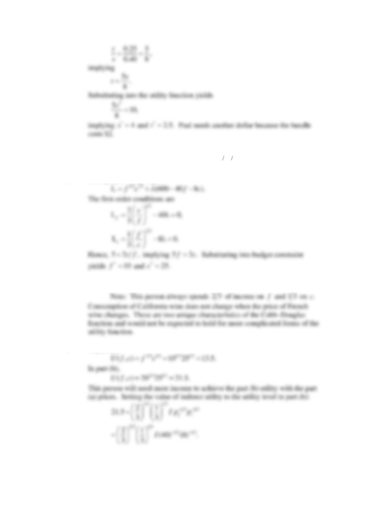
4.2 Use a simpler notation for this solution:
2 3 1 3
( , )U f c f c=
and
600.I=
a. Setting up the Lagrangian:
b. With the new constraint,
*20f=
and
*25.c=
c. In part (a),
Chapter 4: Utility Maximization and Choice
26
4.3 Given
22
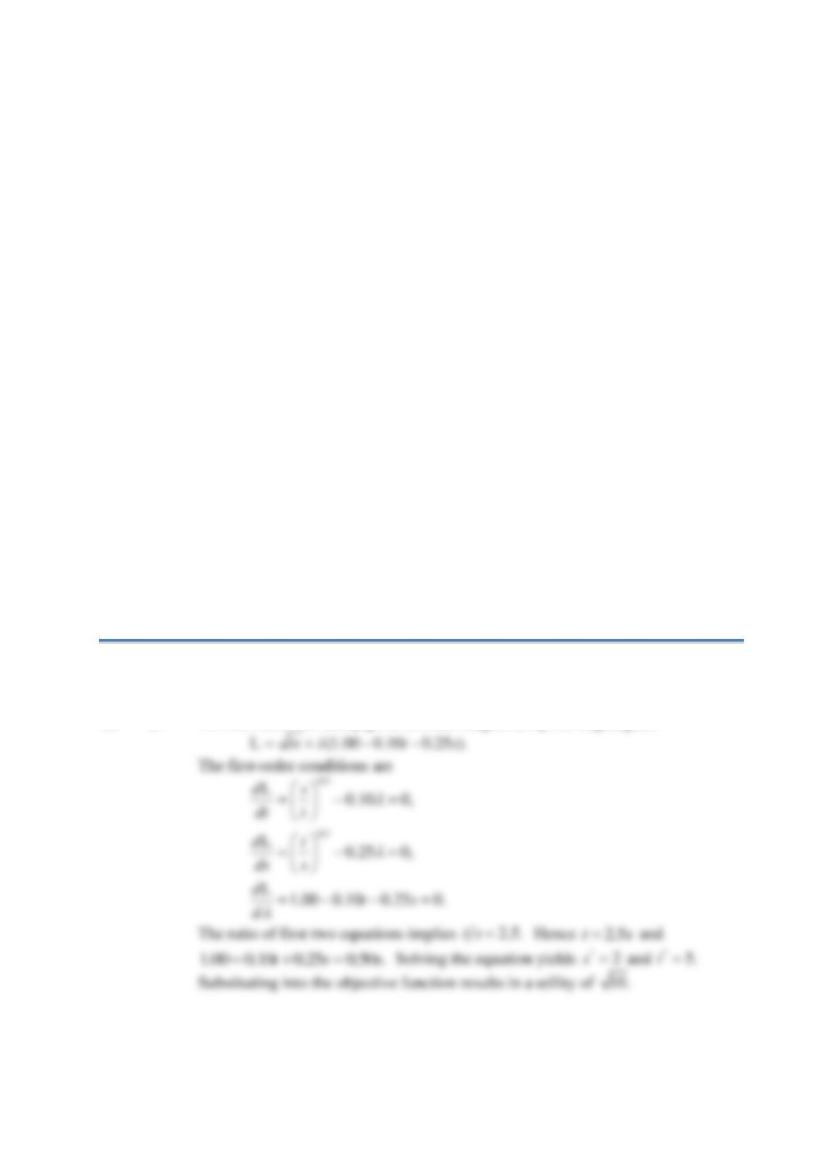
( , ) 20 18 3 .U c b c c b b= − + −
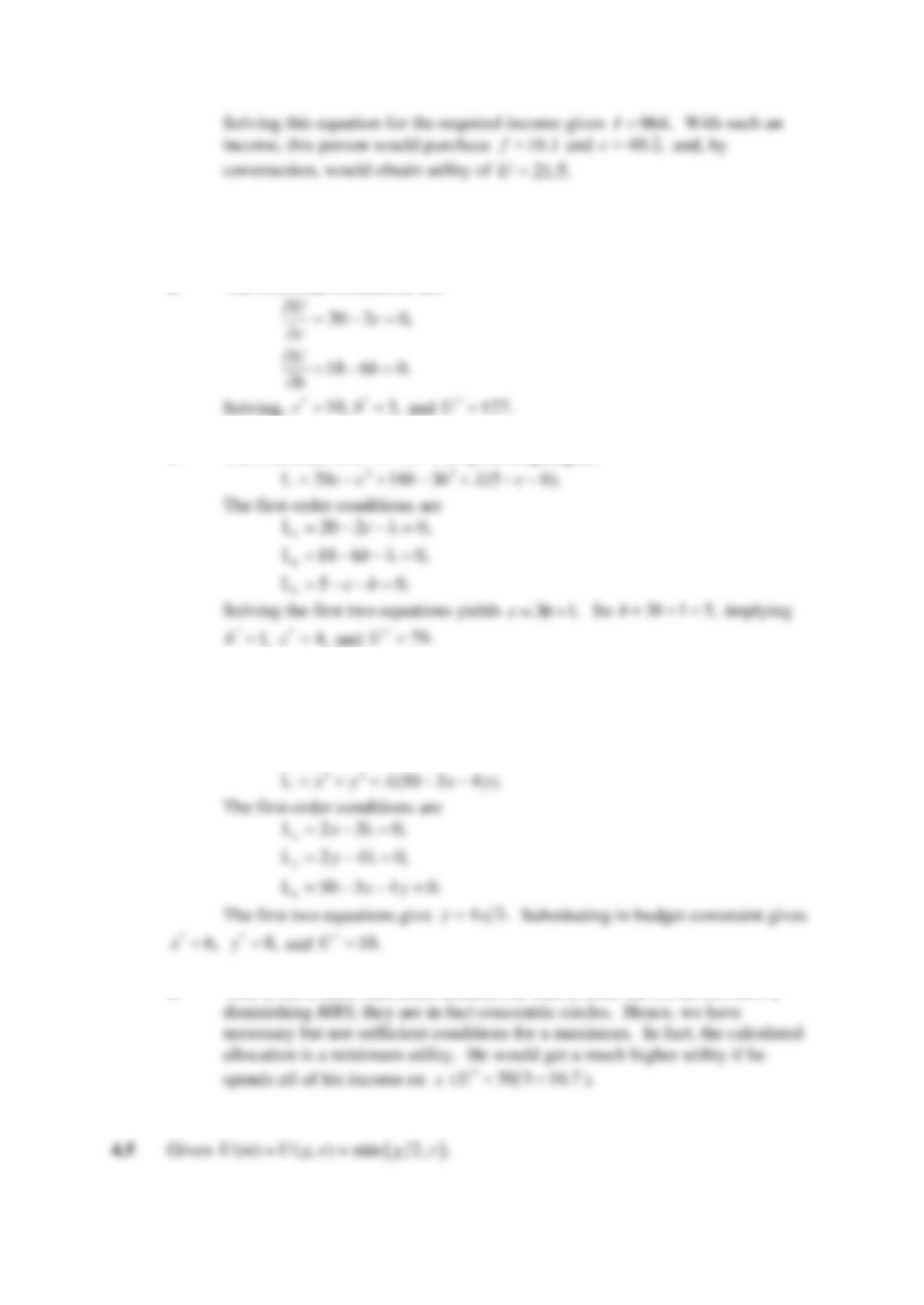
a. The first-order conditions are
b. The constraint is
5.bc+=
Set up the Lagrangian:
4.4 Given
2 2 0.5
( , ) ( ) .U x y x y=+
Note that maximizing
2
U
will also maximize
.U
a. The Lagrangian is
b. This is not a local maximum because the indifference curves do not have a
Chapter 4: Utility Maximization and Choice
27
a. No matter what the relative prices are (i.e., the slope of the budget constraint),
b. Substituting
2gv=
into the budget constraint yields
2,
gv
p v p v I==
or
c. Since
2,U g v==
indirect utility is
d. The expenditure function is found by interchanging
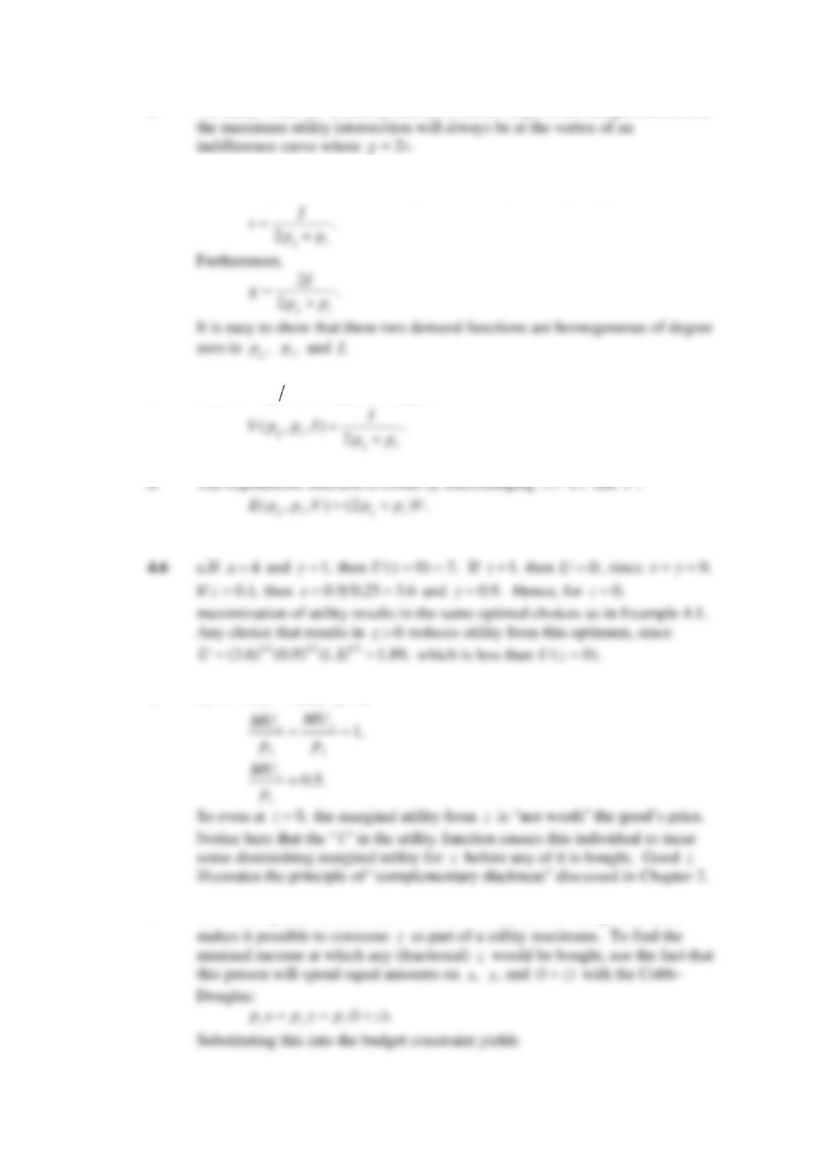
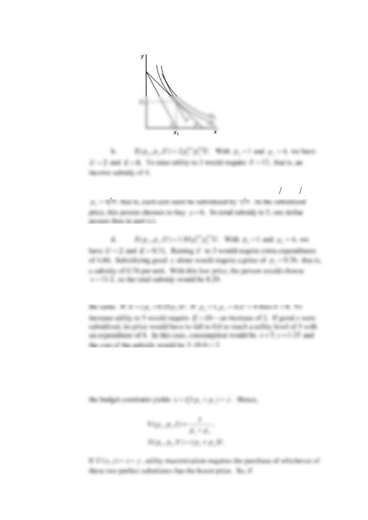
4.6 a.If
b. At
4,x=
1y=
, and
0.z=
c. If
10,I=
optimal choices are
16,x=
4,y=
and
1.z=
A higher income
Chapter 4: Utility Maximization and Choice
28
Chapter 4: Utility Maximization and Choice
29
4.7 a.
c. Now we require
0.5 0.5
8 2 4 3
x
Ep= =
or
0.5 8 12 2 3.
x
p==
So
e. In the fixed proportions case, an income grant and a price subsidy would cost
4.8
a. If
( , ) min( , )U x y x y=
, utility maximization requires
xy=
. Substitution into
Chapter 4: Utility Maximization and Choice
30
b. It is interesting that the discontinuous utility function has continuous indirect
4.9 Given
( , ) .U x y ax by=+
There are two cases to consider. First, assume
Analytical Problems:
4.10 Cobb–Douglas utility
a. The demand functions in this case are
Chapter 4: Utility Maximization and Choice
31
4.11 CES utility
a. For utility maximization,
b. If
0,
=
c. Part (a) shows
Chapter 4: Utility Maximization and Choice
32
Hence,
or
4.12 Stone–Geary utility
a. For
0,xx
utility is negative, so the individual will spend
0x
px
first. With
b. Calculating budget shares from part (a) yields
Chapter 4: Utility Maximization and Choice
33
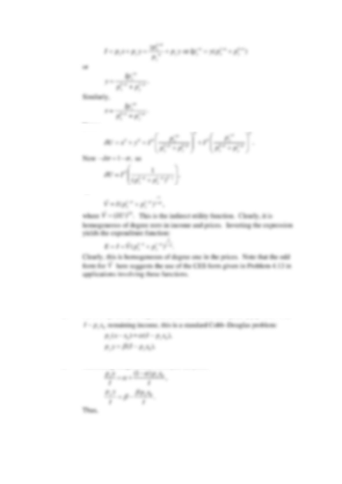
4.13 CES indirect utility and expenditure functions
a. Given
1
( ) .U x y
=+
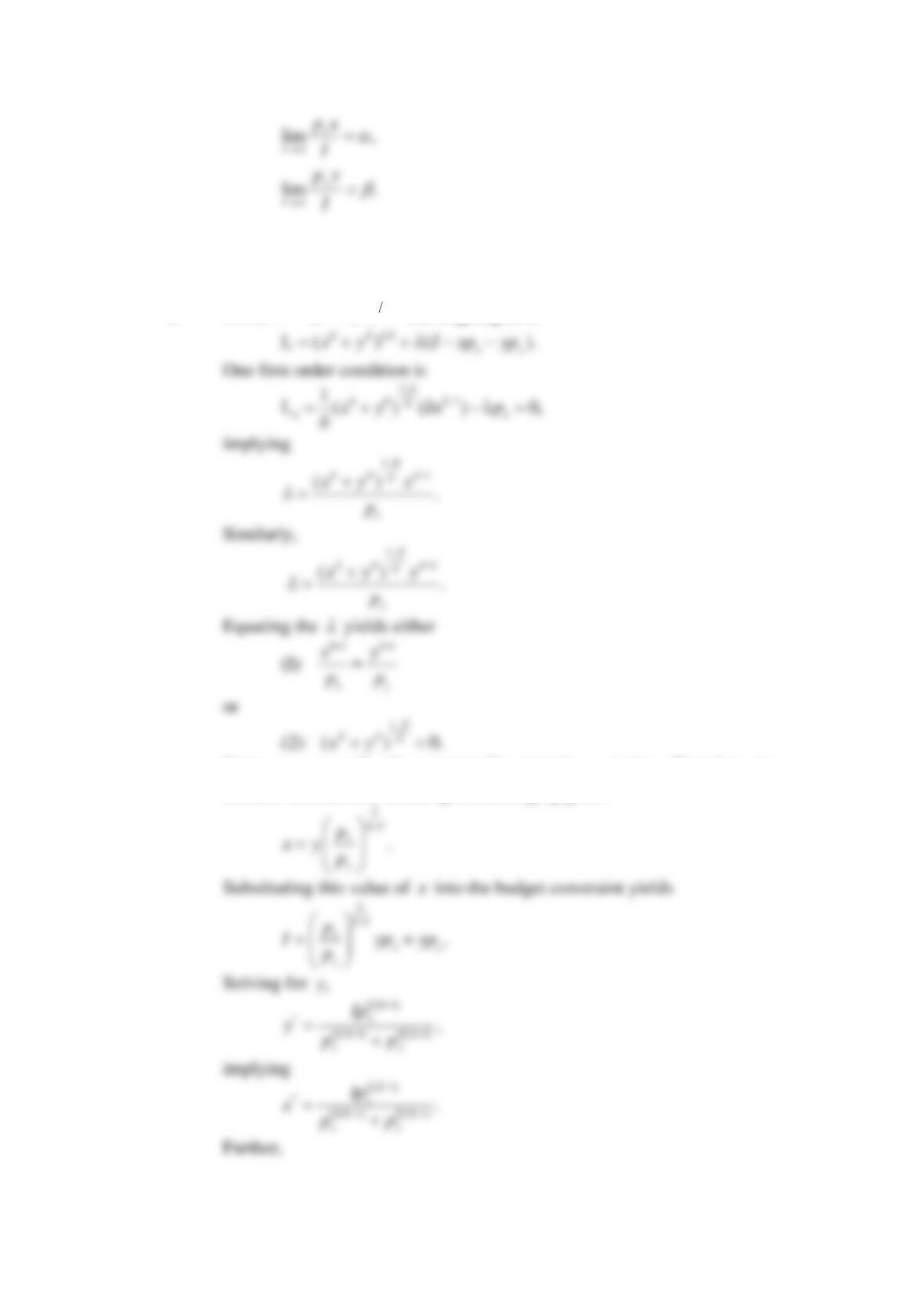
The Lagrangian is
Since we assume
0,U
equation (2) cannot be a solution. Therefore, the
solution satisfies (1), which upon rearranging gives
Chapter 4: Utility Maximization and Choice
34
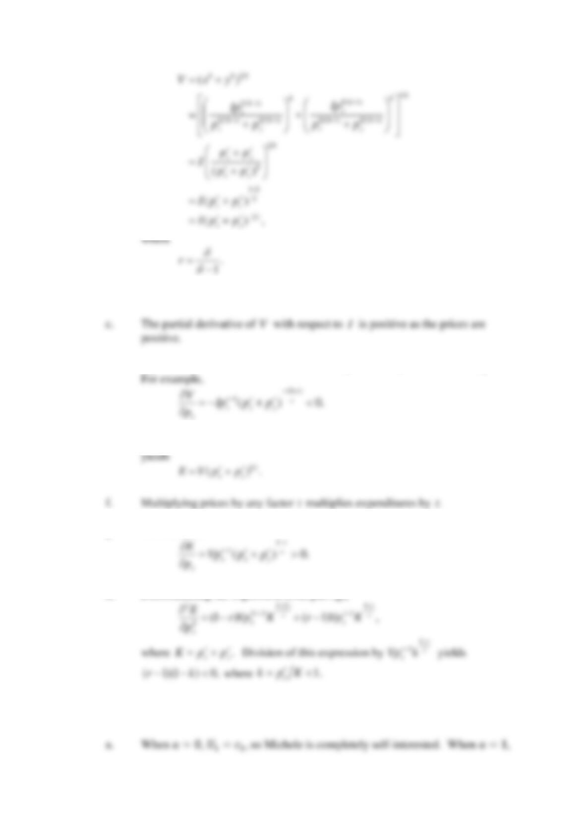
b. Scale all variables by
t
V
and the function is unchanged.
d. Again, the partial derivatives of
V
with respect to the prices are both negative.
e. Simply reversing the positions of
V
and
I
in the indirect utility function
g. For example,
h. Differentiating the expression from part (g),
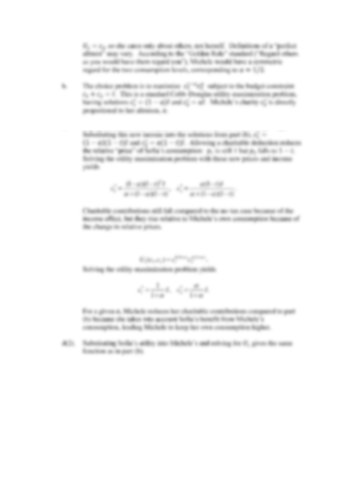
4.14 Altruism
Chapter 4: Utility Maximization and Choice
35
c. A proportional income tax just reduces her net income from 𝐼 to (1 − 𝑡)𝐼.
d(1). Substituting Sofia’s utility function into Michele’s and solving for 𝑈1 yields