Review Problems 95
43
1
3
y
vv
. Substituting gives
2
43 13 43
11
33
x
vv v v
x
, or 2
3
vvx
x
, a line-
ar equation for v as a function of x. An integrating factor is given by
28. We first rewrite the differential equation for 0x as
2
12
x
e
yy
x
x
, showing that the
x
29. We first rewrite the differential equation for 1
2
x as
12
121
21
yyx
x
, show-
ing that the equation is linear. An integrating factor is given by
30. The expression
xy
suggests the substitution vx
y
, which implies that yvx,
and thus that 1yv
. Substituting gives 1vv
, or 1vv
, a separable equa-
tion for v as a function of x. Separating variables gives 1
1dv dx
v
. The further
96 Chapter 1: First-Order Differential Equations
31. Rewriting the differential equation as 22
321
y
xy x
shows that it is linear. An inte-
grating factor is given by
3
2
exp 3
x
x
dx e
, and multiplying the equation by
gives 333
22
321
x
xx
eyxey xe
, or
x
33
2
21
x
x
D
ey xe
. Integrating then leads to
32. We first rewrite the differential equation as
3
dy
x
yy
dx
, showing that the equation is
separable. For 1y separating variables gives 3
1dy x dx
yy
, and the method of
partial fractions yields
x
x
y
x
x
x
D
y
Review Problems 97
33. Rewriting the differential equation for ,0xy in differential form gives
22
32 4 0xydxxydy
,
and because
22
32 4 4
x
yy xy
yx
, the given equation is exact. We apply the
method of Example 9 in Section 1.6 to find a solution in the form
,Fxy C. First, the
x
y
x
y
x
solution
2
3
21
y
x
C
x
, or finally 23
2
y
xx C, as found above.
Still another solution arises from writing the differential equation for ,0xy as
1
13
24
dy x
y
y
dx x
, which shows that it is Bernoulli with 1n . The substitution
2
vy implies that 12
y
v and thus that 12
1
2
y
vv
. Substituting gives
12 12 12
113
22 4
x
vv v v
x
, or 13
2
x
vv
x
, a linear equation for v as a function of x.
x
x
98 Chapter 1: First-Order Differential Equations
34. Rewriting the differential equation in differential form gives
33 0x y dx x y dy,
and because
33 3
x
yxy
yx
, the given equation is exact. We apply the
x
g
x
Alternatively, rewriting the given equation for ,0xy as
13
3
y
dy
x
y
dx
x
shows that it is
homogeneous. Substituting y
v
x
then gives 13
3
dv v
vx
dx v
, or
261
3
dv v v
xdx v
.
x
35. Rewriting the differential equation as
2
21
1
dy x y
dx x
shows that it is separable. For
1y separating variables gives 2
12
11
x
dy dx
yx
, or
2
ln 1 ln 1yxC ,
x
Review Problems 99
36. Rewriting the differential equation for 0x
, 01y as cot
dy
x
dx
yy
shows
that it is separable. The substitution 2
y
u gives
12
ln 1 ln 1
1
dy du u y
u
yy
,
leading to the general solution
ln 1 ln sinyxC
, or
sin 1
x
yC
, or final-
ly
2
csc 1yC x.
Alternatively, writing the differential equation for 0x
, 01y as
y
x
y
101
CHAPTER 2
MATHEMATICAL MODELS AND NUMERICAL
METHODS
SECTION 2.1
POPULATION MODELS
Section 2.1 introduces the first of the two major classes of mathematical models studied in the
textbook, and is a prerequisite to the discussion of equilibrium solutions and stability in Section
2.2. In Problems 1-8 we find the desired particular solution and sketch some typical solution
curves, with the desired particular solution highlighted.
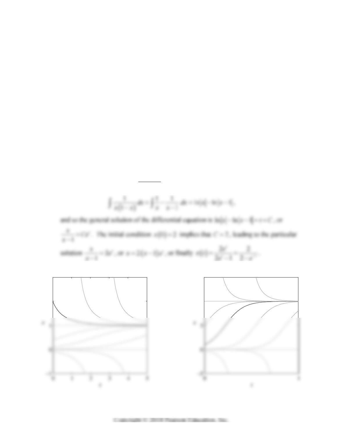
1. Separating variables gives
1
1dx dt
xx
. By the method of partial fractions
2
3
Problem 1
10
15
Problem 2
102 Chapter 2: Mathematical Models and Numerical Methods
2. Separating variables gives
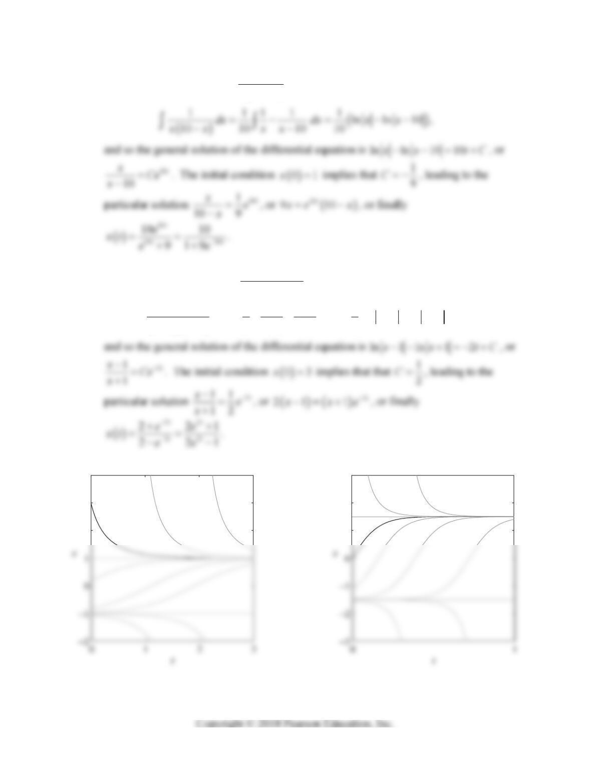
1
10 dx dt
xx
. By the method of partial fractions
3. Separating variables gives
1
11
dx dt
xx
. By the method of partial fractions
11111
ln 1 ln 1
11 2 1 1 2
dx dx x x
xx x x
,
2
3
4
Problem 3
1
2
3
Problem 4
Section 2.1: Population Models 103
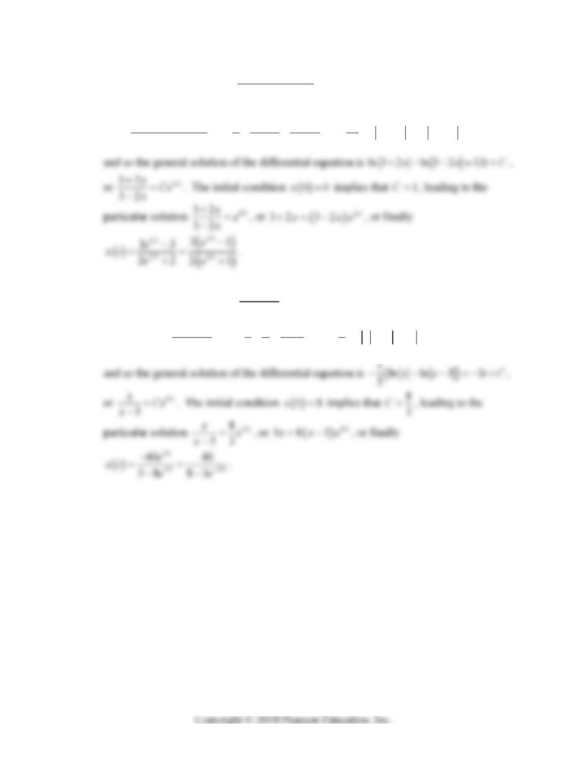
4. Separating variables gives
1
32 32 dx dt
xx
. By the method of partial
fractions,
11111
ln 3 2 ln 3 2
32 32 6 32 32 12
dx dx x x
xx x x
,
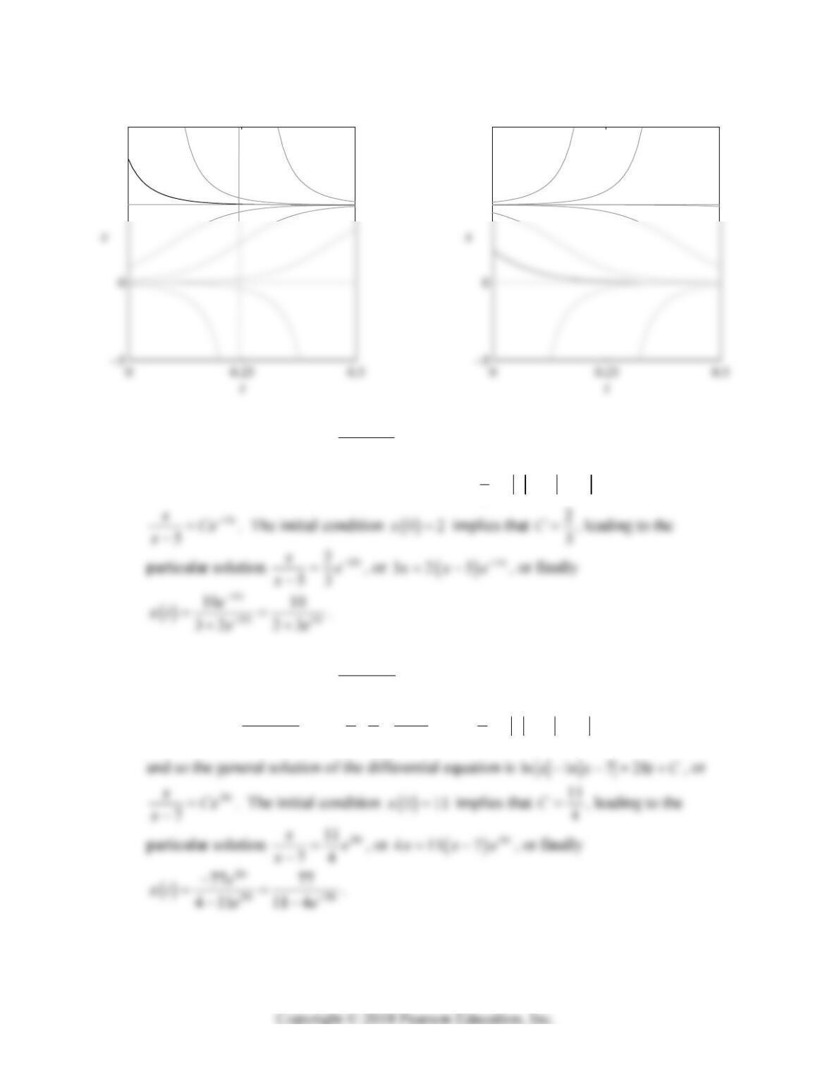
5. Separating variables gives
13
5dx dt
xx
. By the method of partial fractions,
11111
ln ln 5
55 55
dx dx x x
xx x x
,
104 Chapter 2: Mathematical Models and Numerical Methods
5
10
Problem 5
5
10
Problem 6
6. Separating variables gives
13
5dx dt
xx
. Using the partial fraction expansion
found in Problem 5, we find the general solution
1ln ln 5 3
5
x
xtC
, or
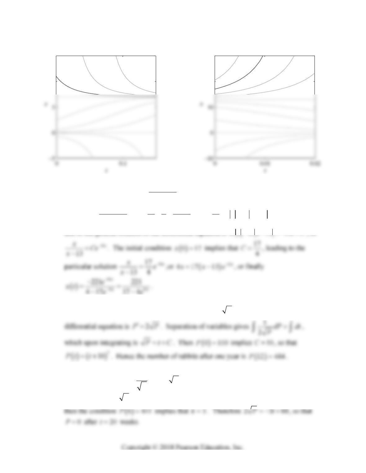
7. Separating variables gives
14
7dx dt
xx
. By the method of partial fractions,
11111
ln ln 7
77 77
dx dx x x
xx x x
,
Section 2.1: Population Models 105
10
15
Problem 7
20
30
Problem 8
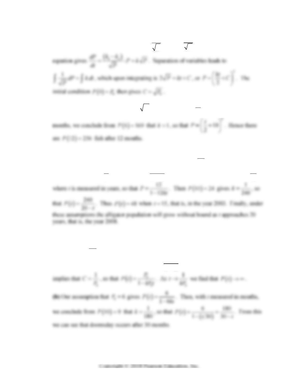
8. Separating variables gives
17
13 dx dt
xx
. By the method of partial fractions,
11111
ln ln 13
13 13 13 13
dx dx x x
xx x x
,
9. Substitution of
0 100P and
020P into PkP
yields 2k, so the
10. Given that k
PP PkP
p
, separation of variables and integration as in
Problem 9 yields 2PktC . The initial condition
0900P gives 60C, and
106 Chapter 2: Mathematical Models and Numerical Methods
11. (a) Substituting our assumptions that 1
k
p
and 2
k
P
into the general population
(b) Our assumption implies that 010CP
, so that
2
10
2
kt
P
. Measuring t in
12. Separating variables in our assumption that 2
PkP
gives 2
1dP k dt
P
, which upon
integrating leads to 1kt C
P
, or 1
PCkt
. Now
012P implies that 1
12
C,
13. (a) Substituting our assumptions that 1
kP
and 2
kP
into the general population
equation gives
2
12
dP kkPPkP
dt
, where 12
0kk k
by our assumption that
. Solving as in Problem 12 leads to 1
PCkt
. The initial condition
0
0PP
Section 2.1: Population Models 107
14. Now 2
dP kP
dt with 0k, and solving once again leads to
0
0
1
P
Pt kP t
. As t
the rabbit population P approaches zero, because k is negative.
0
0
16. The relations in Problem 15 give 0
22
61
120 2400
D
kP
and a limiting population of
17. The relations in Problem 15 give 0
22
0
12 1
240 2400
D
kP
and a limiting population of
00
9 240 180
12
BP
MD
rabbits. The solution is then
18. Writing dP b
aP P
shows that the limiting population M is b
19. The relations in Problem 18 give 0
22
0
10 1
100 1000
B
kP
and 00
0
9 100 90
10
DP
MB
.
Problem 33 below then gives the solution
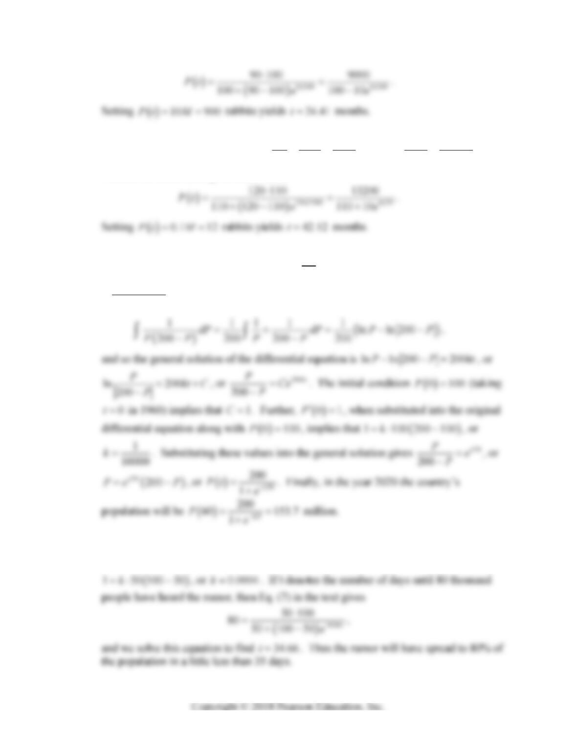
108 Chapter 2: Mathematical Models and Numerical Methods
20. The relations in Problem 18 give 0
22
0
11 1
110 1100
B
kP
and 00
0
12 110 120
11
DP
MB
.
Problem 33 below then gives the solution
21. Separating variables in our assumption that
200
dP kP P
dt
gives
1
200 dP k dt
PP
. By the method of partial fractions
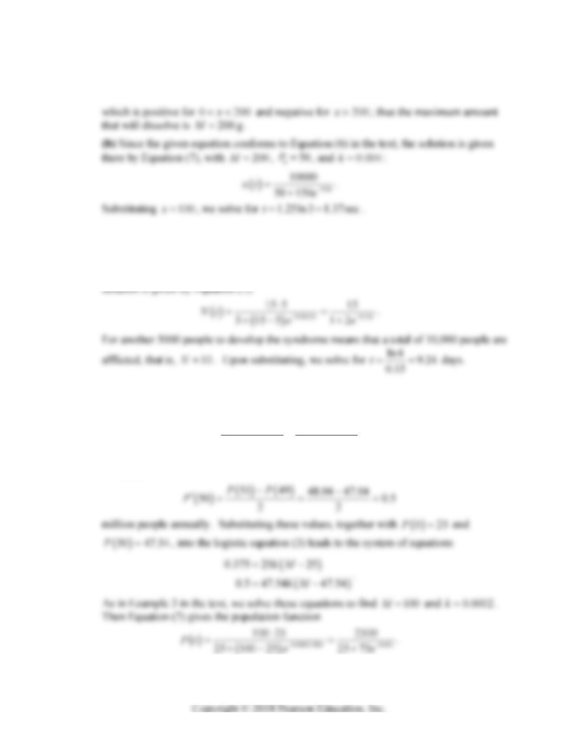
22. We work in thousands of persons, and so take 100M for the total fixed population.
Substituting this together with 050P and
01P into the logistic equation gives
Section 2.1: Population Models 109
23. (a) The given differential equation implies that
2
0.8 0.004 0.004 200
x
xx xx
,
24. Our assumptions imply that
15Nt kN N
, where we measure N in thousands of
people. Substituting
05N and
00.5N gives 0.01k. With N in place of P,
this is the logistic initial value problem in Equation (6) of the text (using 15M), so its
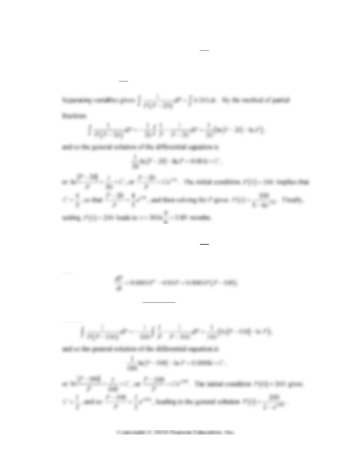
25. (a) Following the suggestions (and thus taking 0t in 1965), we estimate the rate of
population growth in 1965 to be
11
25.38 24.63
00.375
22
PP
P
million people annually. The corresponding estimate for the year 2015, corresponding to
50t, is
(b) We find that 75
P
when 50ln 9 110t
, that is, in 2075 A.D.
110 Chapter 2: Mathematical Models and Numerical Methods
26. Our assumptions lead to the differential equation 2
0.001
dP PP
dt
for the rodent
population
Pt. Substituting
0100P and
08P gives 0.02
, and so
2
0.001 0.02 0.001 20
dP PP PP
dt
.
8
27. Our assumptions lead to the differential equation 20.01
dP kP P
dt for the animal
population
Pt. Substituting
0200P and
02P, we find that 0.0001k, so
that
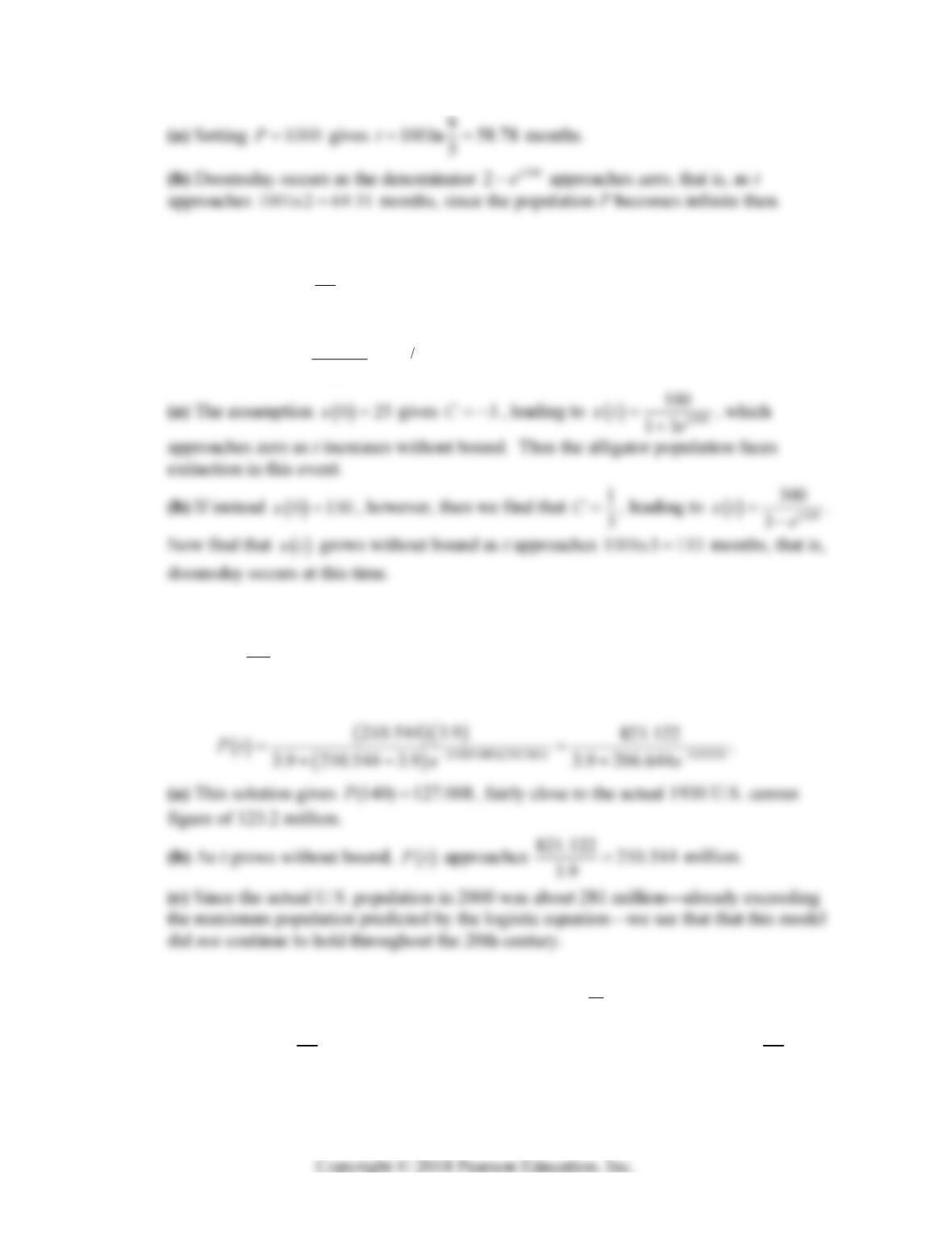
Separating variables gives
10.0001
100 dP dt
PP
. By the method of partial
fractions
Section 2.1: Population Models 111
28. Our alligator population satisfies the equation
2
0.0001 0.01 0.0001 100
dx xx xx
dt
.
With x in place of P, this is the same differential equation as in Problem 27, and so our
general solution is 100
100 t
xCe
x
, as found there.
29. Here we have the logistic equation
2
0.03135 0.0001489 0.0001489 210.544
dP PP PP
dt
,
where
0.0001489k and 210.544P. With 03.9P as well, Eq. (7) in the text gives
30. Separating variables in the differential equation gives 0
1t
dP e dt
P
, with general
solution 0
ln t
PeC
. The initial condition
0
0PP gives 0
0
lnCP
,
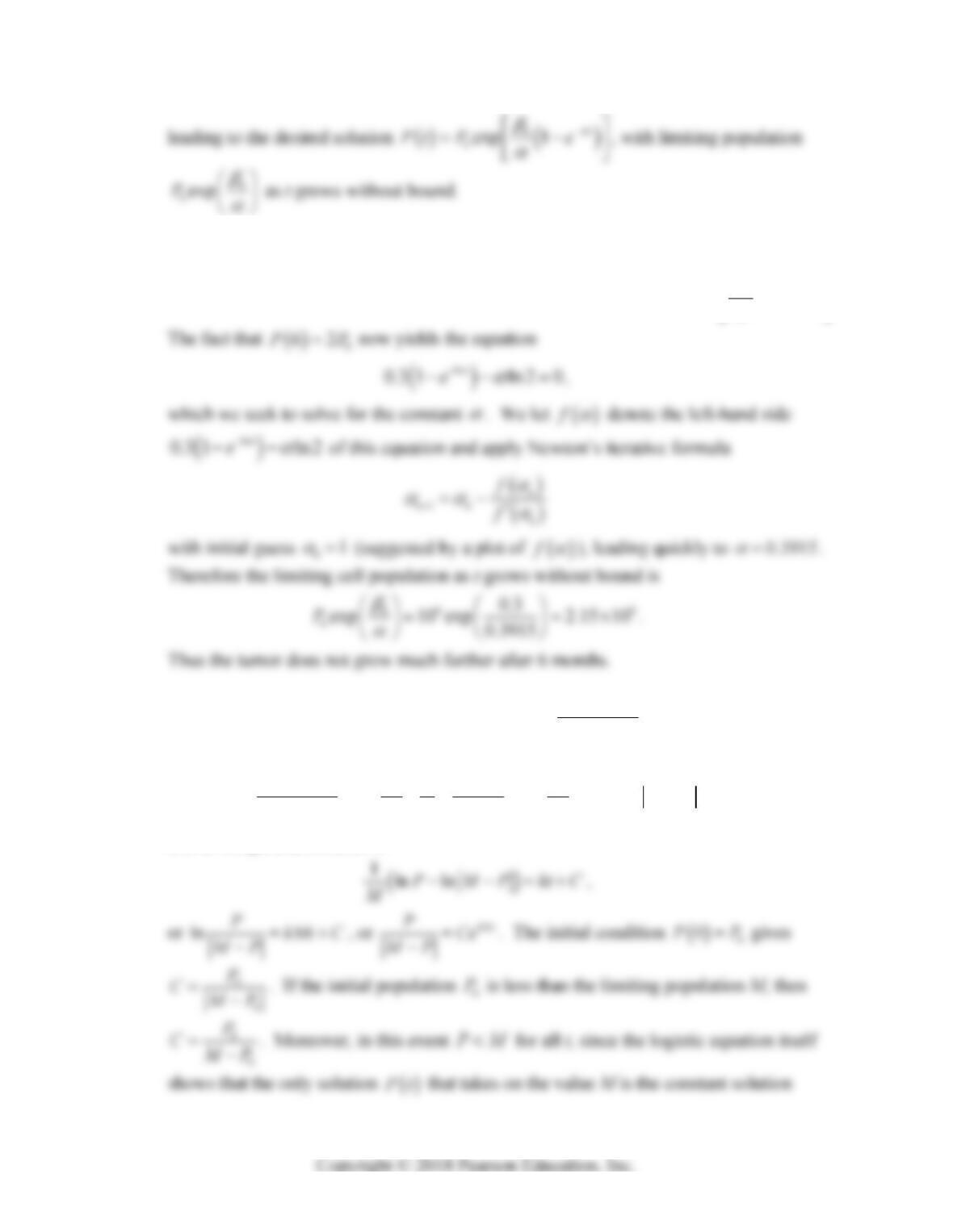
112 Chapter 2: Mathematical Models and Numerical Methods
31. Substituting
6
010P and
5
0310P into the differential equation
0
t
Pt e P
yields 00.3
. Hence the solution given in Problem 30 is
0
0.3
exp 1 t
Pt P e
.
32. Separating variables in the logistic equation gives
1dP k dt
PM P
. By the
method of partial fractions
11111
ln lndP dP P M P
PM P M P M P M
,
and so the general solution is
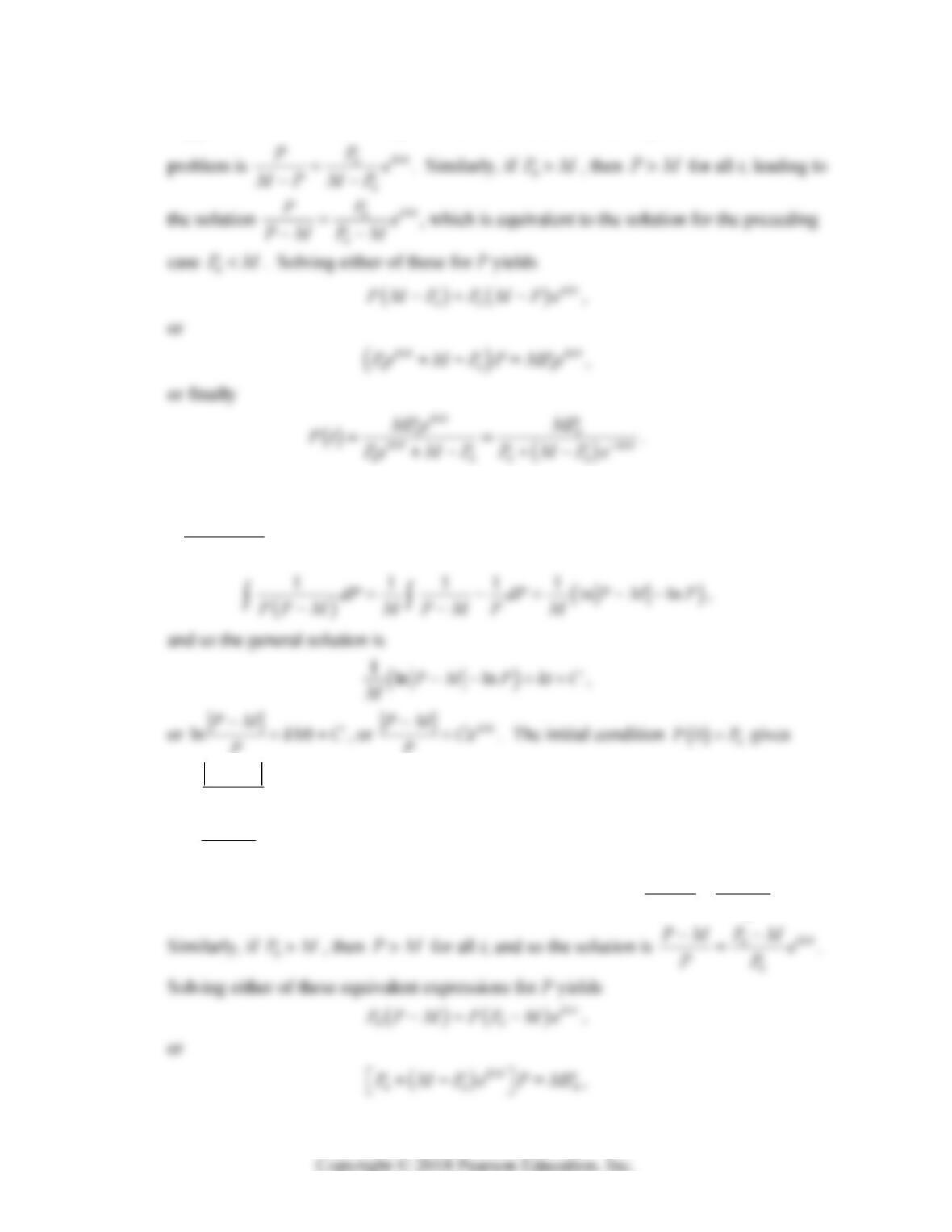
Section 2.1: Population Models 113
Pt M. It follows that if 0
PM, then the solution of the logistic initial value
P
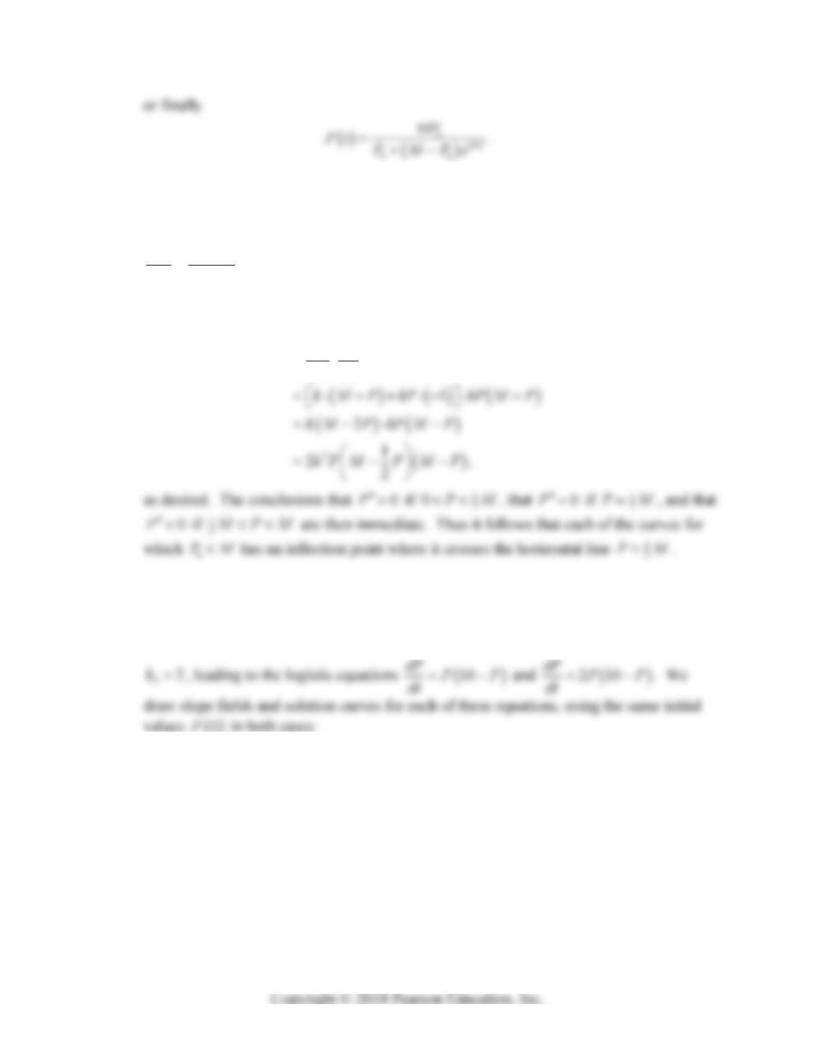
33. (a) Separating variables in the extinction-explosion equation gives
1dP k dt
PP M
. By the method of partial fractions
P
P
0
0
PM
CP
. If the initial population 0
P is less than the threshold population M, then
0
0
M
P
CP
. Moreover, as in Problem 32, in this case
P
M for all t. Thus for 0
PM
the solution of the extinction-explosion initial value problem is 0
0
kMt
MP MP
e
PP
.
P
114 Chapter 2: Mathematical Models and Numerical Methods
(b) If 0
PM, then the coefficient 0
M
P is positive and the denominator increases
without bound, so
0Pt as t But if 0
PM, then the denominator
00
kMt
PPMe approaches zero—so
Pt —as t approaches the positive value
0
0
1ln P
kM P M from the left. Thus the population either becomes extinct or explodes.
34. Differentiation of both sides of the logistic equation
PkPMP
yields
M
dP dP
PdP dt
35. Any way you look at it, you should conclude that the larger the parameter 0k, the
faster the logistic population
Pt approaches its limiting population M:
To examine the question geometrically, we will assume that 10M and that 11k and